
Abstract
Ancient murals are of high artistic value and boast rich content. The accurate classification of murals is a challenging task for researchers and can be arduous even for experienced researchers. The image classification algorithms currently available are not effective in the classification of mural images with strong background noise. A new multichannel separable network model (MCSN) is proposed in this study to solve this issue. Using the GoogLeNet network model as the basic framework, we adopt a small convolution kernel for the extraction of the shallow-layer background features of murals and then decompose larger, two-dimensional convolution kernels into smaller convolution kernels, for example, 7 × 7 and 3 × 3 kernels into 7 × 1 and 1 × 7 kernels and 3 × 1 and 1 × 3 kernels, respectively, to extract important deep-layer feature information. A soft thresholding activation scaling strategy is adopted to enhance the stability of the network during training, and finally, the murals are classified through the softmax layer. A minibatch SGD algorithm is employed to update the parameters. The accuracy, recall and F1-score reached 88.16%, 90.01%, and 90.38%, respectively. Compared with mainstream classification algorithms, the model demonstrates improvement in terms of classification accuracy, generalizability, and stability to a certain extent, supporting its suitability in efficiently classifying murals.
Introduction
Ancient murals are known for their precious artistic value. The structural layout, character depictions, delineation, coloring and pigmentation in murals systematically reflect the artistic styles of muralists across different historical periods, the ideas of artistic inheritance and evolution and the history of the exchange and integration of Chinese and Western art [1, 2]. Researchers are eagerly seeking ways to quickly identify issues regarding research value and academic interest in different types of ancient mural images. Mural classification enables researchers to select different types and styles of mural images. However, due to the multitudinous types of murals and their respective characteristics, artificial mural classification is time consuming, arduous, and low in accuracy. Computer-aided mural classification gradually emerged in the 1990s [3]. For instances, with the aid of computer technology, Tompa et al. [4] recognized and classified coin-type ancient artifacts; Bhaumik et al. [5] summarized the application of computer technology in Buddhist iconography, such as gesture recognition and the superresolution reconstruction of the images; and Chpmtip and Natdanai [6] used genetic algorithm to recognize Buddhist amulets. The use of digital technology can effectively promote the study of mural classification, not only improving its efficiency and accuracy but also advancing progress in ancient mural research.
Computer-aided technology has made considerable contributions to improving the research value of murals. Cao et al. [7] used a dark channel prior and the retinex theory to repair soot-covered mural images, and Li et al. [8] employed a generation-discriminator network model under deep learning in the repair of damaged murals. Many researchers have made great contributions to the classification of murals. For example, Zeng et al. [9] classified and then repaired damaged mural areas. Yang et al. [10] categorized the artistic styles of murals from different dynasties, finding, for example, that murals of different dynasties differ in decorations and backgrounds. Tang et al. [11] studied similarity metrics between images based on the overall contour structures and proposed a scale-invariant feature transform (SIFT) algorithm to remove noise murals by extracting feature vectors in the murals irrelevant to various scale transformations from images and classifying murals in combination with a support vector machine. However, this method was affected by the number of murals to be classified, and the classification effect was not desirable. Starting from the character style of ancient murals, Hao et al. [12] divided murals into different categories of art characteristics from different dynasties, such as images, costumes, and headwear of uncovered individuals. Kumar et al. [13] used pretrained AlexNet and VGGNet models to extract features and classify murals to address insufficiency of existing mural datasets. As murals contain much background noise, feature extraction directly influences the quality of the classification. Wang et al. [14] transformed the classification of mural pigments into a multispectral image classification for categorizing ancient mural pigments.
As computer technology [15,16,17] continues to develop, deep learning has progressed by leaps and bounds, and the powerful feature extraction ability of the convolutional neural network has been applied in various image processing tasks, particularly displaying good performance in classification tasks. Krizhevsky et al. [18] devised the AlexNet neural network model used for image classification. This model won the 2012 ImageNet ILSVRC championship. ALexNet has 8 layers of neural networks in total, including 5 convolutional layers and 3 fully connected layers. The classification effect for mural images is acceptable for relatively simple backgrounds. However, for mural images with complex texture features, the classification effect is inadequate. The 2014 ILSVRC runner-up, the VGG network [19,20,21], includes two versions, i.e., VGG16 and VGG19, both with powerful extraction capacities. Simply increasing the number and depth of network layers in the VGG network architecture can improve the performance of the network. However, for mural images, deep-layer networks are prone to overfitting, leading to low network performance. In 2014, GoogLeNet [22] won the ILSVRC championship. It substitutes the average pooling layer to replace the fully connected layer that causes the greatest parameter overhead and replaces the simple convolutional layer with an inception module. In addition, it uses 1 × 1 convolution for dimension reduction operations. Since the implementation of GoogLeNet, the classification accuracy of deep learning has rivaled that of humans. In 2015, ResNet [23, 24] won the championship for classification tasks, surpassing human cognition with an error rate of 3.75%, and created a new model record for 152-layer network architectures. However, when dealing with mural classification tasks, network models with excessively deep layers may extract extra, irrelevant noise and feature information, causing a reduction in the classification accuracy.
Given the strong background noise contained in murals, the complexity of desirable mural features and the characteristics of network models’ ability to extract features in deep learning, we aim to design a network model suitable for mural classification. Therefore, using the ImageNet GoogLeNet network model as the basic framework for the mural classification task, we propose a new multichannel separable network (MCSN) model. The innovations of the proposed model are as follows. (1) It expands the number of network channels and decomposes larger, two-dimensional convolution kernels into two smaller convolution kernels to extract deep-layer mural features so that the network can focus on the content of the mural itself and reduce the interference on feature extraction by the background noise in the mural. (2) The activation scaling strategy [25, 26] is used in the network. Each module is multiplied by an activation constant β to increase the stability of the network during training prior to concatenation. (3) In the small batch classification task, a minibatch SGD is used to optimize the parameter equalization to improve network performance. The abovementioned improvements finally help boost the accuracy of neural networks in mural image classification.
Methodology
GoogLeNet network structure
The GoogLeNet model is a convolutional neural network consisting of 22 layers. Its structure is shown in Table 1. The inception structure [27, 28] is introduced to the GoogLeNet model to improve its feature extraction ability. The core idea here is to approximate and cover the dense structure obtained into an optimized local sparse structure.
In the inception structure, the sizes of the convolutional kernels are specified as 1 × 1, 3 × 3, and 5 × 5 to avoid the issue of patch alignment. Furthermore, the above three convolution kernels are stacked on each other to output different results. However, a reduction in the aggregation of the convolution kernels in space allows the model to extract abstract mural feature information at a deeper level. One solution is to increase the number of 3 × 3 and 5 × 5 convolutional kernels in the higher layers to obtain a larger area of features. However, this may cause a series of problems, such as greatly augmenting the computational overhead in the mural classification process. A second solution is to output the convolution and pooling operations in parallel before they are combined. However, this will not only increase the number of output values but also cause the optimized sparse structure to be covered, resulting in a computational explosion. A third solution is to introduce a 1 × 1 convolutional kernel following the convolution and prior to the pooling and arrange them in parallel. Although this could generate a good effect to a certain extent, the resulting large convolutional kernel will cause an increase in the number of parameters required by the network, also resulting in a large number of computations. Given these issues in the above methods, we decompose the large convolution kernels in the Inception layers into two smaller convolution kernels when we make improvements to the network structure in this study. In this way, the number of computations is reduced during the mural classification process while ensuring that the extracted mural features are be lost, thereby improving the accuracy of mural classification.
Multichannel separable network model (MCSN)
Overall network design
The MCSN model is shown in Fig. 1. The design criteria of the model are as follows. First, the depth and width of the model should moderately increase or decrease while ensuring that information is not lost. In the front part of the network structure, the mural image does not directly pass through a highly compressed layer. Instead, the dimensionality of the incoming feature map is slowly reduced to avoid creating bottlenecks in information representation. In the intermediate stage of the network, a low-dimensional convolution kernel is used for aggregation in space so that the mural feature information is compressed simply while guaranteeing information integrity and training speed.

The structure of MCSN
Utilizing the entirety of the mural feature data and a binary file with corresponding labels, the MCSN model passes one set of mural feature data (input as a three-channel, 299 × 299 matrix) into six size 3 × 3 convolution kernels, where the mural edge and the low-level line features are extracted first. Then, the extracted information enters 3 modules A successively, where the model extracts the local frame, namely, higher-level features, i.e., the uniquely styled curves and fine textures of the mural. Then, the output is passed through 5 modules B. In the Concat operation within module B, the data is multiplied by an activation scaling constant β to stabilize the network training. This module extracts the content specific to the target mural. The color and content information of more complex murals can be extracted through 2 modules C. However, this part requires a combination of additional mural datasets to fully identify the specific mural image. Then, the data is passed to an average sampling pooling layer with a window size of 8. Finally, there are two fully connected layers that implement the dropout layer during training. This can not only reduce the number of network computations but also prevent overfitting. Finally, automatic feature extraction is completed in the MCSN model. The last fully connected layer classifies the eight kinds of extracted mural feature vectors and calculates the probability value of the mural label of the sample through the softmax function, as shown in Eq. (1).
In this study, we calculate the degree of approximation between the mural label predicted by the network and the actual label by designing a loss function based on cross entropy, as shown in Eq. (2):
To enhance the generalizability of the network and prevent overfitting, the marginal effect of the dropout label is added to Eq. (2) to regularize the classifier layer and smooth the predicted mural labels calculated by the network. The smoothing parameter is set to ε, and the formula for calculating the actual label is:
The predicted label distribution calculated by the network is:
Then, the following cross entropy gradient formula is used:
This ensures confidence in the predicted results from the model, making the predicted label approximate the actual label as much as possible. In this experiment, the number of mural categories K = 8, and ε is set to 0.1.
Improvements
-
1.
Introduction of the adaptive separation convolution module to extract deep features from murals. The MCSN model proposed in this study introduces the adaptive separation convolution module to improve the model’s ability to extract deep features, reduce the number of computations and enhance network performance. The decomposition process breaks down an n × n convolution kernel into two one-dimensional convolution kernels, a 1 × n and an n × 1 kernel. First, by transforming one n × n convolution kernel into two one-dimensional convolution kernels, the number of parameters in the network is reduced, thereby speeding up network computations. Second, the number of channels in the model is expanded by arranging one n × n convolution kernel in parallel into a 1 × n and an n × 1 convolution kernel. This change increases the number of network layers, which improves the nonlinearity of the network; furthermore, a BN layer and the ReLU nonlinear activation function are included in each added layer so that the model can adapt to changes in gradients and perform computations quickly. Therefore, the model exhibits good performance in feature extraction [29]. A large number of experiments have demonstrated that a network with excessively deep layers will trigger the disappearance or explosion of the back-propagation gradient. Underlying the propagation method is chain derivation, which involves a series of multiplication operations. When the network is overly deep and the majority of the multiplication factors are smaller than 1, then the result of the multiplications approaches 0, causing the gradient to disappear. In contrast, when the multiplication factors tend to infinity, a gradient explosion will occur [30,31,32]. To address the gradient explosion problem, each module B is multiplied by an activation scaling factor. Three types of adaptive separation convolution modules, A, B, and C, are designed based on this rule, as shown in Figs. 2, 3, and 4.
Fig. 2 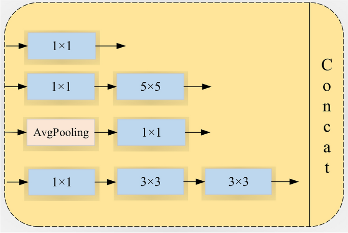
Adaptive separation convolution module A
Fig. 3 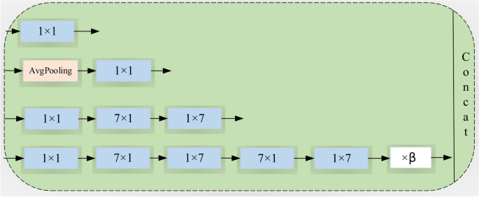
Adaptive separation convolution module B
Fig. 4 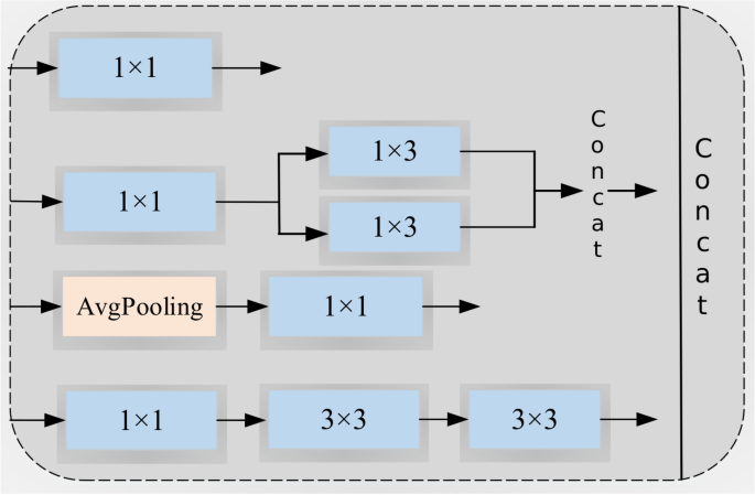
Adaptive separation convolution module C
The adaptive separation convolution module B in Fig. 4 is used as an example to validate the effect of the reduced computations after the convolution kernel is separated in this study. For example, the size of the feature map input to this layer is 28 × 28 × 256, and 128 7 × 7 convolution kernels are needed. All convolution kernels in this layer use the same padding to ensure that the size of the feature map output remains constant. Although numerous convolution kernels are added to this module, the complexity of the parameter computation is optimized through the dimensionality reduction method in the study. We take the abovementioned 128 7 × 7 convolution kernels as an example. First, 128 1 × 1 convolution kernels are added to the branches of the 7 × 7 convolution kernel, and then, while ensuring that the receptive field remains unchanged, the 7 × 7 convolution kernel is decomposed into two, one-dimensional kernels of sizes 7 × 1 and 1 × 7. The calculation formulas for the parameters before and after this operation are shown in Eqs. (6) and (7).
Before separation:
$$28^{2} \times 7^{2} \times 256 \times 96 \, = \, 9.4 \times 10^{8} .$$(6)After separation:
$$28^{2} \times 1^{2} \times 256 \times 64 + 28^{2} \times 7 \times 1 \times 64 \times 128 \times 2 = 1.3 \times 10^{8} .$$(7)From the above results, it is obvious that after the convolution separation operation performed in this study, the required parameters decrease by more than 7 times, significantly reducing the number of computations and the size of the convolution kernel.
-
2.
Introduction of the minibatch SGD algorithm to optimize the network. SGD randomly selects only one sample in each iteration to calculate the gradient. Multiple samples can be randomly sampled uniformly in each iteration to form a minibatch, which is then used to calculate the gradient [33]. The advantages of minibatch SGD are as follows. (1) Within a reasonable range, the memory utilization rate and the parallel efficiency of large matrix multiplication are improved. (2) The number of iterations needed to run an epoch (full dataset) is reduced, and the processing for the same amount of data is further accelerated. (3) Within a certain range, generally speaking, a larger Batch_Size means a more accurate definite descending direction and a smaller ensuing training shock.
The minibatch SGD algorithm is described as follows: suppose the objective function \(f\left( x \right):{\mathbb{R}}^{d} \to {\mathbb{R}}\). The time step before the iteration starts is set to 0. The independent variable of the time step is denoted as \(x_{0} \in {\mathbb{R}}^{d}\), which is usually obtained by random initialization. In each time step t > 0 that follows, the minibatch SGD randomly and uniformly samples a minibatch βt, comprised of the training data sample indexes. We can obtain each sample in the minibatch by sampling with or without replacement. The former allows multiduplicated samples in the same mini-batch, while the latter does not, which is more common. For any of these two methods, Eq. (8) can be used:
$$g_{t} \leftarrow \nabla f_{{\beta_{t} }} (x_{t - 1} ) = \frac{1}{|\beta |}\sum\limits_{i \in } {\nabla f_{i} (x_{t - 1} )} .$$(8)This equation can be used to calculate the gradient \({\text{g}}_{t}\) at \(x_{t - 1}\), the objective function at which the mini-batch \(\beta_{t}\) is located with time step tt. Here, \(\beta_{t}\) represents the batch size, namely, the number of samples in the minibatch, and is a hyperparameter. Similar to the stochastic gradient, the minibatch stochastic gradient gt obtained by sampling with replacement is also an unbiased estimate of the gradient \(\nabla f\left( {x_{t - 1} } \right)\). Given learning rate ηt (which always takes a positive number), the iteration of the minibatch SGD to the independent variable is shown in Eq. (9):
$$x_{t} \leftarrow x_{t - 1} - \eta_{t} g_{t} .$$(9)It is impossible to reduce the variance of the gradient obtained based on random sampling in the iterative process. Therefore, in practice, either the learning rate of minibatch SGD self-attenuates in the iterative process (for example, ηt = ηta, ηt = ηat), or the learning rate attenuates once every several iterations. In this way, the variance of the product of the learning rate and the minibatch stochastic gradient will diminish. The genuine gradient of the objective function is always applied in gradient descent during the iterative process, without any need to self-attenuate the learning rate.
-
3.
Introduction of a soft thresholding activation scaling strategy to increase network stability. Generally, as ancient mural images are derived from data in the real world, they contain noise or redundant information to varying degrees. In a sample, any information irrelevant to the classification task of the current model can be regarded as noise or redundant information. In particular, the background noise in murals will undermine the learning effect of the network model. To address the impact of noise, inspired by the deep residual shrinkage network, which integrates soft thresholding in the network as a nonlinear transformation, we perform soft thresholding in our network; the resulting relationship between the input x and the output y following soft thresholding is shown in Fig. 5a. Soft thresholding directly assigns a zero value to features whose absolute value is less than a certain threshold and contracts other features tending to zero within a certain range. Figure 5b shows the partial derivative of the input y with regard to the input x. The gradient value of the soft thresholding function is either 0 or 1, similar to the characteristics of the ReLU activation function. This characteristic can expose the model to risks such as gradient disappearance and gradient explosion during the training process of the model.
Fig. 5 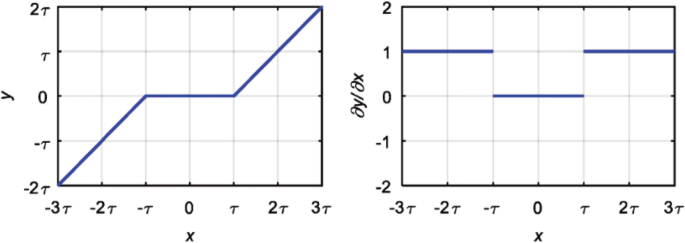
Principle of soft thresholding. a Soft thresholding. b Partial derivative
According to this mechanism, after adaptive separation module B extracts features through two separation methods, the activation scaling strategy is applied for soft thresholding of the network. First, the features obtained by adaptive separation module B are multiplied by an activation scaling factor β (a coefficient ranging between 0 and 1). Based on various experiments from previous researchers, the activation scaling factor β is often set to 0.2, which is neither too large to exert a significant impact on the network nor too small to cause a dramatic change in the gradient. This method ensures not only that all thresholds are positive but also that they are not too large and will not render all outputs zero. Therefore, it ensures network stability during training and optimal performance of the model.


Algorithm steps and processes
The algorithm of the MCSN neural network for mural classification is divided into three stages: data preprocessing, mural dataset training, and mural dataset testing. We adopted training/validation/testing splitting rather than k-fold cross validation for mural dataset division because our focus was on the images for which the classification accuracy was low. Based on the classification outcomes, we adjusted the hyperparameters to achieve the purpose of model optimization.
The overall flow chart of the algorithm is shown in Fig. 6.

Algorithm flow chart
The specific steps of the algorithm are as follows:
-
Input: Mural dataset.
-
Output: Optimal network model.
-
Step 1. The datasets are divided into three groups using the random sampling method: a Train dataset, a Val dataset and a Test dataset.
-
Step 2. Convert the data set in Fig. 7 into tfrecords format, as shown in Fig. 7.
Fig. 7 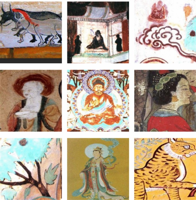
tfrecords conversion chart. a Mural data set, b binary conversion diagram
-
Step 3. The Train and Val datasets are fed to the network in batches.
-
Step 4. Weights, bias values and other parameters are initialized, completing the preparation work.
-
Step 5. The network model is trained to extract the features of the mural images.
-
Step 6. Minibatch SGD is used to continuously update and optimize the parameters. The network model is saved every 2000 times until it converges.
-
Step 7. The saved model is used for classification on the Test dataset to find the best network model.
-
Step 8. A comparison experiment is conducted for the best network model.

Experimental results and discussion
Experimental environment and design
Hardware environment: CPU: Inter Core i7-7700 K, memory: 16 GB, graphics card: NVIDIA GeForce GTX 1080Ti.
Software environment: TensorFlow, which is the basic framework of deep learning. This framework supports not only distributed computing models but also other algorithms in addition to deep learning and is characterized by a strong transfer ability and easy extensibility. C++, Python, Java, and other programming languages can be adopted to the front end, which is responsible for the design of calculation graphs, while the back end executes the calculation graphs by providing a running environment.
The mural materials used in the training and testing dataset in this study come from the scanned versions of the Complete Collection of Dunhuang Murals in China and Tomb Murals Unearthed Along the Silk Road in China. These murals covering a variety of themes and originate from the Sui, Tang, Ming and Qing dynasties and other dynasties that scholars investigate in their studies. After consulting relevant research experts, we roughly classify the murals initially into 8 categories for the classification experiments: people, plants, pusa (bodhisattva), animals, buildings, clouds, disciples, and fo (Buddhas). In this experiment, each type of mural dataset is divided into two groups: one group of data is used for training, and the other group is used for testing. The original dataset contains a total 2607 images, including 425 of fo, 375 of pusa, 400 of disciples, 420 of people, 312 of clouds, 345 of animals, 335 of plans and 295 of buildings. Due to the limited size of the dataset, we adopt a number of data enhancement methods to expand the dataset, including scaling, brightness transformation, noise addition, flipping, etc. The final dataset used in this experiment includes 11,630 images. The data after enhancement are divided into the training dataset and the testing dataset according to a ratio of 8:2, and the distribution of the mural datasets is shown in Table 2.
To ensure that the training model has good generalizability, it is necessary to set an appropriate learning rate and number of categories. The parameter batch_size is set to 16 to strengthen the network training speed. In addition, the keep_pro hyperparameter is set to 0.5 to improve the generalizability of the model by eliminating some of the background features of the murals when extracting data during the training process. Minibatch SGD is used to update and optimize the parameters using the following formula:
A batch size of 16 is used to approximate the gradient of the entire training dataset, after which parallel computing is carried out with the following formula:
The parameters used in the experiment are shown in Table 3.
Experimental analysis and comparison
To validate the efficiency and use value of the model in this study, we conduct the research from six aspects, namely, validation of the effect of the soft thresholding activation scaling strategy, analysis of the feature maps extracted by the proposed algorithm versus other algorithms, comparison of the combined effect of different adaptive separation convolution modules, qualitative and comparative analysis using different algorithms, quantitative and comparative analysis of the experimental data, and analysis of misclassified murals.
Validation of the effect of the soft thresholding activation scaling strategy
The soft thresholding activation scaling strategy affects model learning, that is, it impacts the accuracy of mural recognition to a certain extent. To validate the effect of the activation scaling strategy in the MCSN neural network model, five experimental groups are used for comparison, namely, an experimental group without a scaling factor and experimental groups with separate scaling factors of 0.1, 0.2, 0.4, and 0.6. The above five groups of variables are set to be trained in the MCSN model, and then 20 murals are randomly selected from the 8 categories to validate the classification accuracy. A comparison of the classification accuracies observed after these 5 groups of variables are trained is shown in Fig. 8.

Comparison of classification accuracies for different activation factors
Figure 8 shows that the classification accuracy of the model without the activation factor is 72.51% after training, increasing slightly after an activation factor is used. When β = 0.2, the classification accuracy is highest, at 86.36%. Therefore, after incorporating an activation factor, the MCSN model has an improved classification accuracy, and optimal classification is achieved when parameter β is set to 0.2.
Analysis of feature maps extracted by the proposed algorithm versus other algorithms
To further validate the MCSN model’s ability to extract mural features, the feature maps extracted by the MCSN model are compared with those extracted by mural classification algorithms in references [12,13,14] and those extracted by GoogLeNet and the classical VGG algorithm, as shown in Fig. 9.

Comparison of mural feature extraction under different algorithms
As shown in Fig. 9, an observation of the faces of mural figures reveals that the feature maps extracted by the algorithms in references [12,13,14] are blurred, and texture details are missing. Traditional convolutional neural networks such as GoogLeNet display a poor ability to extract mural features. Although the VGG network model can extract complete mural features, its performance is not as good as that of the MCSN model in extracting local features. Therefore, it is validated that the MCSN model shows a better ability to extract mural features and is suitable for mural classification.
Comparison of the combined effect of different adaptive separation convolution modules
To find the optimal number of adaptive separation convolution modules A, B, and C, 8 groups with different combinations of adaptive separation convolution modules A, B, and C for each group are set for training, as shown in Table 4. Their accuracies are reported in Fig. 10.

Comparison of classification accuracy values for different module combinations
In Fig. 10, when 5 modules B are used, that is, for Group 1 to Group 4, the accuracy ranges between 83 and 87%, and the changes in the number of modules A and C have little impact. When the number of modules B is 3, 4, or 6, as in Group 5 to Group 8, the accuracy decreases to 76–80%, and the changes in the numbers of modules A and C still have little impact on the accuracy. Therefore, it can be inferred that the number of modules B has the greatest effect on the performance of the network. Therefore, Group 2 is the optimal combination of adaptive separation convolution modules A, B, and C; that is, 3A + 5B + 2C has the highest accuracy after training.
Qualitative and comparative analysis
To validate the effectiveness of the model under special circumstances in this study, a qualitative and comparative analysis of different algorithms is conducted by manipulating two qualitative image parameters, namely, brightness and similarity. Eight categories of murals are selected in the experiment to validate the classification effect of the MCSN algorithm. Figures 11, 12, and 13 show mural classification test results using the mural classification algorithms in references [12,13,14], GoogLeNet, the classic VGG algorithm and the MCSN model.

Murals with different brightness levels

Single-channel histogram and dHash combined comparison chart

Comparisons of the accuracy, recall, and F1-score of the different algorithms
Due to differences in the real world environments of mural images, for example, the sunshine to which the Dunhuang murals are exposed and the dark environment in which tomb murals are kept, we select mural images of different brightness level for comparison to verify the classification results from the different algorithms. Generally, the average brightness of an image should be 128, ranging within [100,150] for photographs taken normally. In Fig. 11, three types of images with a brightness of 46.19 (dark), 115.35 (normal), and 167.77 (overexposed) are selected to investigate the mural classification ability of the models. The resulting accuracies are shown in Table 5.
As shown in Table 5, the algorithm in this study still achieves good performance in the recognition of mural images taken in dark, normal brightness and overexposed environments. The algorithm in [12] classifies murals according to costumes, and the algorithm in [13] classifies murals according to color, both of which are sensitive to brightness. Therefore, the accuracy of classification for these two algorithms is poor when the mural is in an environment that is too dark or too bright. The algorithm in [14] has good accuracy under normal brightness and overexposed brightness conditions, but its recognition ability suffers in dark environments. The two classic algorithms have poor adaptability and exhibit low accuracy under dark environments. As the impact of brightness on the accuracy of mural classification is taken into consideration during data enhancement, the model proposed in this study has better generalizability. Therefore, its prediction accuracy is also higher than that of the other algorithms.
The image similarity is jointly determined by the color in the image and the image fingerprint and is represented by the degree of coincidence of the single channel histogram and the difference hash algorithm (dHash), respectively. In the dHash algorithm, a smaller value (which ranges between 0 and 64) means a higher similarity; that is, in terms of the Hamming distance, the dHash algorithm determines how different the 64-bit hash value is between two images. The value of the single channel histogram is 0–1, and a greater value indicates to a higher similarity. A combination of the two can better judge the recognition effect of the classification algorithm. In Fig. 12, the image coincidence degrees are (left to right) 0.51, 0.48 and 0.66. The dHash values are 29, 30, and 27, respectively. A comparison chart for the combination of the single channel histogram and dHash is shown in Fig. 12. The accuracies are shown in Table 6.
It is clear in Table 6 that when the histogram coincidence degree and dHash value are the same, the classification accuracy for people in reference [12] is the highest owing to its strong ability to extract color features from murals. Compared with other algorithms, the MCSN model also maintains a good classification ability when the intracluster variation is minimal, demonstrating that the network model proposed in this study performs better than classic classification algorithms.
The algorithm in this study achieves very good classification results because in the convolutional neural network, a large convolution kernel is decomposed into two small convolution kernels. Despite the increase in network nonlinearity, the mural features extracted are not lost in the deep network, and this operation enables the decision function in the network to achieve better performance by playing the role of implicit regularization. However, the algorithms in references [12, 13] achieve good performance in the classification of murals with colorful costumes and rich colors. Under certain circumstances, such as extreme brightness and similarity between murals, their classification accuracy does not reach the level of the algorithm proposed in this study, as they fail to extract information well. Although the algorithm in reference [14], GoogLeNet, and VGG the network use higher-layer networks, they are not as robust to images displaying the above phenomena and thus fail to achieve the desired classification effect. In conclusion, the model proposed in this study is highly accurate in the recognition of images with these phenomena, demonstrating the feasibility of the proposed model and its good prospect for application to mural classification.
Quantitative and comparative analysis
To further test that the model proposed in this study has an obvious effect in the identification of massive mural images, we perform a quantitative and comparative analysis of the performance of the algorithms in references [12,13,14], the GoogLeNet algorithm and the VGG algorithm on the mural datasets described in Table 2. Statistical analyses and calculations are carried out for the gradient orientation histogram input to a small part of the local area of the image, and the obtained features are applied to the BP network for classification. The recognition accuracy values of the above five algorithms are compared with that of the algorithm proposed in this study, as shown in Table 7. The single-category recognition accuracy of the model proposed in this study is calculated as:
where mi represents the total number of correctly predicted category labels (calculated by Eq. (1)) consistent with the actual labels, i.e., the correct number in this category; Mi is the total number of samples in this category; and i is the category to which it belongs. Then, the recognition accuracy is:
where N is the total number of samples, and n is the total number of categories, that is, 8. It is clear in Table 7 that although the algorithms in references [12,13,14] exhibit a higher average recognition rate than the other classic algorithms, they do not have strong generalizability, nor do they have good adaptability to mural images taken under special circumstances. For large-scale and complex mural images, other deep learning algorithms do not perform as well as the algorithm proposed in this study, in that they extract a large amount of information on mural features and are less accurate. In addition, for the same mural images photographed with a low illumination intensity and at low resolution, the recognition rate of the algorithm proposed in this study is better by 6% and 5%, respectively, than that of the algorithms in [12, 13] and by 7–14% than that of the classic algorithms. The accuracy of the proposed model in mural recognition is increased to 90.38% by using methods such as convolution decomposition, introduction of the activation scaling factor, and parameter optimization, demonstrating the effectiveness and advantages of the model.
In addition, three indicators, i.e., accuracy, recall, and F1-score, commonly used to assess the performance of different algorithms, are adopted to comprehensively evaluate the performance of the algorithm proposed in this study, as shown in Fig. 13. The recall and F1-score are specifically defined as:
where TP is a correctly predicted positive sample, FP is a negative sample incorrectly predicted as a positive sample, and FN is a positive sample incorrectly predicted as a negative sample.
The comparisons of recall and F1-score in Fig. 13 also reveal that the model proposed in this study displays better performance than the other models. In terms of the recognition of massive mural images by the different algorithms, particularly in the recognition of target murals with drastic differences in information content, such as images with information distributed globally or locally, the algorithm proposed in this study selects an appropriate convolution kernel size in the convolution operation. As the traditional GoogLeNet algorithm may encounter certain bottlenecks when extracting features from a large dataset and fail to process a large amount of data, it is not highly workable in this aspect. The loss functions of ResNet and VGG constantly oscillate and are unable to achieve high accuracies either. The algorithms in references [12,13,14] do not have good generalizability and fail to classify murals photographed in harsh environments. Their indicators are not as desirable as the algorithm proposed in this study. The algorithm in this study increases the network depth by decomposing a large convolution kernel into two smaller convolutions kernels and avoids overfitting. The introduction of the activation scaling factor into module B ensures smooth convergence in the later stage of training and improves the recognition accuracy.
Analysis of misclassified murals
During the experiment, since murals contain multiple objects, some classification errors can occur during the classification process, as shown in Fig. 14.

Misclassified murals
In Fig. 14a, the mural category is “animals”. However, the two images are incorrectly classified as “people” (left) and “plants” (right). Because the person on horseback and the plant beneath the bird have more features than the horse and the bird itself, respectively, the algorithm cannot detect the category of the mural well. In Fig. 14b, the mural category is “buildings”. However, as the buildings depict human-like features, they are mistakenly classified into the “people” category. Similarly, the mural category in Fig. 14c is “plants”, yet they are mistakenly assigned into the “building” category, as the architectural features behind the plants are obviously more prominent than the plant features. Due to the above problems, the classification effect for murals with multiple categories is not as good as that for single-category murals. Therefore, further research is necessary to improve the classification for these multiple-category murals.
Conclusions
In this study, we designed an MCSN mural classification model based on deep learning, which targeted at the classification of murals under the influence of complex environment, such as illumination and mural similarity. The results showed that this model improved the efficiency and accuracy of mural classification, and therefore may serve as a convenient and time-saving method for scholars dedicated to research on the dynasty identification and classification of murals, thereby improving the efficiency of mural classification. Currently, the dynasties and authenticity of historical relics, such as ancient porcelains and costumes, have to be artificially identified by historical relic experts. Inspired by this issue, we applied deep learning in the identification and classification of historical relics. However, to achieve satisfactory outcomes, the problems of dataset selection, image pre-processing and suitable model determination had to be solved.
The MCSN mural classification model proposed in this study reduced the number of computations in feature extraction and improved the classification accuracy of mural images through dimensionality reduction, channel expansion, and parameter optimization. First, the adaptive separation convolution module was used to extract the mural features. A soft thresholding activation factor was introduced into adaptive separation convolution module B to guarantee the stability of the network during training. Due to the small size of the mural datasets, a minibatch SGD algorithm was introduced to optimize the network, and finally, an optimal mural classification network model was obtained. In the experiments, we validated the effectiveness of the MCSN model in mural classification by verifying the effect of the soft thresholding activation scaling strategy, comparing the feature maps extracted by the proposed algorithm with those extracted by other classification algorithms, comparing the combined effect of different adaptive separation convolution modules, performing qualitative and comparative analysis of the experiments using different algorithms, performing quantitative and comparative analysis of the experimental data, and analyzing misclassified murals. Among them, through the qualitative, quantitative and comparative analyses of the feature maps extracted by the various classification algorithms, it is concluded that the neural network proposed in this study can extract abundant features exhibiting a higher classification accuracy. Therefore, the model in this study has a strong learning ability for the murals input into the model and has certain value in practical applications.
The network architecture in this study still has some deficiencies. First, it has low accuracy in the classification of multiple-object murals. For example, when a Buddha image, a bodhisattva image, a plant or an animal is present in a mural, the classification accuracy is low. Therefore, for mural images containing multiple objects, seeking for proper identification and classification models remains necessary. Second, there also exist large-scale murals characterized by multiple categories that are endowed with artistic research value. The single-category classification network cannot classify such murals satisfactorily. Moreover, ambiguities occur when such murals are enlarged. Therefore, in the future, we will focus on collecting large-scale mural images and perform the superresolution reconstruction of the images to optimize them, conduct multiple-category mural classification tasks, and improve the artistic research value of murals. Third, despite the satisfactory performance of the model proposed in this study, its interpretability is poor. The feature maps extracted using traditional methods are blurring, which lack sufficient persuasiveness. Therefore, to validate the performance superiority of the model proposed in this study, gradient-weighted class activation mapping (Grad-CAM) [34] can be used to localize the important predicting regions of the model.”
Availability of data and materials
All data used for analysis in this study are included within the article.
Abbreviations
- MCSN:
-
Multichannel separable network model
References
Ha YP, McDonald N, Hersh S, Fenniri SR, Hillier A, Cannuscio CC. Using informational murals and handwashing stations to increase access to sanitation among people experiencing homelessness during the COVID-19 pandemic. Am J Public Health. 2020;111:E1–3.
Sturdy D. The NHS celebrates its diamond anniversary: In the past 60 years the NHS has continued to improve its care of older people, says Deborah Sturdy. Nursing Older People, 2008, 20(1). https://doi.org/10.7748/nop.20.1.9.s9.
Bird JJ, Faria DR, Manso LJ, Ayrosa PPS, Ekárt A. A study on CNN image classification of EEG signals represented in 2D and 3D. J Neural Eng. 2021;18:026005.
Tompa V, Dragomir M, Hurgoiu D, Neamţu C. Image processing used for the recognition and classification of coin-type ancient artifacts. In: 2017 IEEE Western New York image and signal processing workshop (WNYISPW). IEEE; 2017. p. 1–5.
Bhaumik G, Samaddar SG, Samaddar AB. Recognition techniques in Buddhist iconography and challenges. In: 2018 international conference on advances in computing, communications and informatics (ICACCI). 2018. p. 1285–9. https://doi.org/10.1109/ICACCI.2018.8554780.
Chpmtip P, Natdanai S. Buddhist amulet coin recognition by genetic algorithm. In: Computer science and engineering conference (ICSEC). IEEE; 2013. p. 324–7.
Cao N, Lyu SQ, Hou M, Wang WF, Gao ZH, Shaker A, Dong Y. Restoration method of sootiness mural images based on dark channel prior and Retinex by bilateral filter. Herit Sci. 2021. https://doi.org/10.1186/s40494-021-00504-5.
Li J, Wang H, Deng ZQ, Pan MT, Chen HH. Restoration of non-structural damaged murals in Shenzhen Bao’an based on a generator–discriminator network. Herit Sci. 2021. https://doi.org/10.1186/s40494-020-00478-w.
Zeng F. Research on automatic extraction method of man-made handwriting from mural image. Dissertation. Southwest Jiaotong University; 2011.
Yang B. Research on classification of painting images based on artistic style. Dissertation. Zhejiang University; 2013.
Tang DW, Lu DM, Yang B, et al. Similarity metrics between mural images with constraints of the overall structure of contours. J Image Graph. 2014;18(8):968–75.
Hao YB. Research and Implementation on classification algorithm with people of ancient Chinese murals based on style characteristics. Disseration. Tianjin University; 2017.
Kumar S, Tyagi A, Sahu T, Shukla P, Mittal A. Indian art form recognition using convolutional neural networks. In: Proceeding of 5th international conference on signal processing and integrated networks (SPIN). 2018. p. 800–4.
Wang YN, Zhu DN, Wang HQ. Multispectral image classification of mural pigments based on convolutional neural network. Progr Laser Optoelectron. 2019;56(22):48–56.
Zhou FY, Jin LP, Dong J. A review of the study of reel neural networks. J Comput Sci. 2017;40(06):1229–51.
Chang L, Deng XM. the cosmic neural network in image understanding. J Autom. 2016;42(09):1300–12.
Luo JH, Wu JX. An overview of fine-grained image classification based on depth reuter characteristics. J Autom. 2017;43(08):1306–18.
Krizhevsky A, Sutskever I, Hinton G. ImageNet classification with deep convolutional neural networks. In: Advances in neural information processing systems. SanFrancisco: MorganKaufmann; 2012. p. 1097–105.
Wu J, Min Y. Behavior recognition based on the fusion of 3D-BN-VGG and LSTM network. High Technol Lett. 2020;26(04):372–82.
Gu YF, Liu H. Deep feature extraction and motion representation for satellite video scene classification. Sci China Inf Sci. 2020;63(04):97–111.
Lou GX, Shi HZ. Face image recognition based on convolutional neural network. China Commun. 2020;17(02):117–24.
Christian S, Wei L, Pierrs S, et al. Going deeper with convolutions. In: IEEE conference on computer vision and pattern recognition (CVPR). 2015. p. 1–9.
He KM, Zhang XY, Ren SQ. Deep residual learning for image recognition. In: 2016 IEEE conference on computer vision and pattern recognition (CVPR). IEEE Computer Society; 2016. p. 770–8.
Wang G, Li W, Ourselin S, et al. Automatic brain tumor segmentation using cascaded anisotropic convolutional neural networks. In: International MICCAI brainlesion workshop. Cham: Springer; 2017. p. 178–90.
Wang X, Yu K, Wu S, et al. Esrgan: enhanced su per-resolution generative adversarial networks. In: Proceedings of the European conference on computer vision (S0302-9743). 2019;1113:63–79.
Che CC, Wang HW. Fault diagnosis of rolling bearing based on deep residual shrinkage network. J Beijing Univ Aeronaut Astronaut. 2021;1–10.
Sun L, Jia K, Yeung DY, et al. Human action recognition using factorized spatio-temporal convolution networks. In: IEEE international conference on computer vision. IEEE; 2015. p. 4597–605.
Zheng GY, Han GH, Nouman QS. An inception module CNN classifiers fusion method on pulmonary nodule diagnosis by signs. Tsinghua Sci Technol. 2020;25(03):368–83.
Liu JW, Zhao HD, Luo XL. Research progress of deep learning batch normalization and related algorithms. Acta Autom Sin. 2020;46(06):1090–120.
Liu MF, Wu W, Gu ZH, Yu ZL, Qi FF, Li YQ. Deep learning based on batch normalization for P300 signal detection. Neurocomputing. 2018;275:288–97.
Wu S, Li GQ, Deng L, Liu L, Wu D, Xie Y, Shi LP. L1-norm batch normalization for efficient training of deep neural networks. IEEE Trans Neural Netw Learn Syst. 2019;30(7):2043–51.
Kalayeh MM, Shah M. Training faster by separating modes of variation in batch-normalized models. IEEE Trans Pattern Anal Mach Intell. 2020;42(6):1483–500.
Osawa K, Tsuji Y, Ueno Y, Naruse A, Foo CS, Yokota R. Scalable and practical natural gradient for large-scale deep learning. IEEE Trans Pattern Anal Mach Intell. 2020;99:1–1.
Selvaraju RR, Cogswell M, Das A, Vedantam R, Parikh D, Batra D. Grad-CAM: visual explanations from deep networks via gradient-based localization. Int J Comput Vis. 2020;128(2):336–59.
Acknowledgements
None.
Funding
This work was supported by the Project of Key Basic Research in Humanities and Social Sciences of Shanxi Colleges and Universities (20190130).
Author information
Authors and Affiliations
Contributions
All authors contributed to the current work. JFC devised the study plan, led the writing of the article and supervised the entire process. YMJ, HMC, and MMY conducted the experiments and collected the data, and ZYC performed the analyses. All authors read and approved the final manuscript.
Corresponding author
Ethics declarations
Competing interests
The authors declare that they have no competing interests.
Additional information
Publisher's Note
Springer Nature remains neutral with regard to jurisdictional claims in published maps and institutional affiliations.
Rights and permissions
Open Access This article is licensed under a Creative Commons Attribution 4.0 International License, which permits use, sharing, adaptation, distribution and reproduction in any medium or format, as long as you give appropriate credit to the original author(s) and the source, provide a link to the Creative Commons licence, and indicate if changes were made. The images or other third party material in this article are included in the article's Creative Commons licence, unless indicated otherwise in a credit line to the material. If material is not included in the article's Creative Commons licence and your intended use is not permitted by statutory regulation or exceeds the permitted use, you will need to obtain permission directly from the copyright holder. To view a copy of this licence, visit http://creativecommons.org/licenses/by/4.0/. The Creative Commons Public Domain Dedication waiver (http://creativecommons.org/publicdomain/zero/1.0/) applies to the data made available in this article, unless otherwise stated in a credit line to the data.
About this article

Cite this article
Cao, J., Jia, Y., Chen, H. et al. Ancient mural classification methods based on a multichannel separable network. Herit Sci 9, 88 (2021). https://doi.org/10.1186/s40494-021-00562-9
Received:
Accepted:
Published:
DOI: https://doi.org/10.1186/s40494-021-00562-9
Keywords
This article is cited by
-
Mural classification network based on the fusion of shallow feature enhancement and dense attention aggregation
npj Heritage Science (2025)
-
An algorithm based on lightweight semantic features for ancient mural element object detection
npj Heritage Science (2025)
-
KolamNetV2: efficient attention-based deep learning network for tamil heritage art-kolam classification
Heritage Science (2024)
-
The generation method of orthophoto expansion map of arched dome mural based on three-dimensional fine color model
Heritage Science (2024)
