- Research article
- Open access
- Published:
An adaptive prediction method for mechanical properties deterioration of sandstone under freeze–thaw cycles: a case study of Yungang Grottoes
Heritage Science volume 9, Article number: 154 (2021)
Abstract
Due to the location of the Yungang Grottoes, freeze–thaw cycles contribute significantly to the degradation of the mechanical properties of the sandstone. The factors influencing the freeze–thaw cycle are classified into two categories: external environmental conditions and the inherent properties of the rock itself. Since the parameters of rock properties are inherent to each rock, the effect of rock properties on freeze–thaw degradation cannot be investigated by the control variates method. An adaptive multi-output gradient boosting decision trees (AMGBDT) algorithm is proposed to fit nonlinear relationships between mechanical properties and physical factors. The hyperparameters in the GBDT algorithm are set as variables, and the Sequential quadratic programming (SQP) algorithm is applied to solve the hyperparameter optimization, which means finding the maximum Score. The case study illustrates that the AMGBDT algorithm can precisely determine the effect of each independent factor on the output. The patterns of mechanical properties are similar when the number of freeze–thaw cycles and porosity are used as variables separately and when both are used simultaneously. The uniaxial compressive strength decay rate is positively correlated with the number of freeze–thaw cycles and porosity. The modulus of elasticity is negatively correlated with the number of freeze–thaw cycles and porosity. The results show that the number of freeze–thaw cycles is the main factor influencing the freeze–thaw cycling action, and the porosity is minor. In addition, the fitting accuracy of the AMGBDT algorithm is generally higher than neural networks (NN) and random forests (RF). Studying the influence of porosity and other rock properties on the freeze–thaw cycle will help to understand the failure mechanism of rock freeze–thaw cycles.
Introduction
The Yungang Grottoes, one of the three major grotto groups in China and world-famous stone sculpture art, was inscribed on the UNESCO World Heritage List in 2001. Therefore, Yungang Grottoes has a significant artistic and cultural value. Yungang Grottoes (113°20′ E, 40°04′ N) is located in a continental monsoon semi-arid climate. The annual average temperature in the study area is 7–10 °C, the monthly average temperature in January is − 11.4 °C, and the monthly average temperature in July is 23.1 °C. The freezing period is up to six months, with a standard frozen depth of 1.5 m.
The major stratigraphy of Yungang Grottoes is the Mesozoic Jurassic stratigraphy, mainly composed of fluvial and lacustrine deposits [1]. Yungang Grottoes is distributed in a vast lenticular miscellaneous sandstone. The lithology of the sandstone is mainly calcareous cemented sandstone, and gravel is often visible at the bottom of the sandstone's lenticular body. The main components of the sand are quartz, feldspar, and rock debris. The main components of the conglomerate are quartz breccia, rock clasts, and a small portion of mudstone clumps. Due to the geographical location of the Yungang Grottoes and the environment, the effects of weathering caused by freeze–thaw cycles cannot be ignored.
A number of experiments to investigate the effect of freeze–thaw cycling tests on the mechanical properties of sandstone were conducted [2, 3], such as porosity [4], the number of freeze–thaw cycles [5,6,7]. The water content of the rock and the number of freeze–thaw cycles affect the degree of deterioration by freeze–thaw cycles. The main reasons are as follows. (1) The main cause of freeze–thaw damage in rocks is the repeated generation and dissipation [8] of frost heaving forces. The number of freeze–thaw cycles defines the number of times the frost heaving forces are repeatedly generated and dissipated, which means the more times, the more serious the freeze–thaw damage. (2) Pore water influences rock damage through three mechanisms: phase swelling, hydrostatic pressure, and formation of ice lenses or wedges [9], phase swelling, hydrostatic pressure, and formation of ice lenses or wedges. The mechanisms indicate a positive correlation between the pore water content of rocks and damage to saturated rocks. The larger the initial porosity of the rock, the greater the water content at saturation, resulting in greater tensile stresses in the pore walls caused by volume expansion due to water–ice phase changes. The initial porosity affects the freeze–thaw deterioration of rocks in part.
However, most experiments [10, 11] focused on the effect of external environmental conditions on the freeze–thaw deterioration of sandstone. The mechanism of freeze–thaw damage in rocks shows that the initial porosity of rocks also affects freeze–thaw damage. It is impossible to experimentally achieve the control of variables such as intrinsic rock parameters, which means that it is hard to explore the degree of influence of each variable when multiple variables act. In this paper, with the help of the developed AMGBDT algorithm, we investigate the changes in mechanical properties of sandstone when initial porosity and the number of freeze–thaw cycles are adopted as variables.
The selection of hyperparameters has a significant impact on the fitting performance of GBDT. In this paper, the AMGBDT algorithm is proposed to complete the GBDT hyperparameter tuning task, and a prediction model is given based on this algorithm. The prediction model is based on a series of freeze–thaw cycling experimental data to quantify the extent of porosity effects on rock deterioration under freeze–thaw cycles. The prominent advantage of this method is that the degree of contribution of the rock's inherent parameters to the deterioration can be calculated analytically. This paper provides a considerably more efficient and cost-effective means of studying the failure mechanism of freeze–thaw cycles.
The remainder of this paper is organized as follows. The methodology section introduces the principles of the GBDT algorithm and the SQP algorithm and the construction framework of the AMGBDT-SQP algorithm. The comparison between the fitted curves of experimental data and the AMGBDT algorithm is introduced in the case study when the number of freeze–thaw cycles and the porosity are applied as independent variables separately. The discussion section discusses three methods to demonstrate the GBDT algorithm prediction accuracy by the algorithm Score's evaluation index. The fifth part outlines conclusions.
Methodology
High-accuracy predictions can be obtained by these non-parametric machine learning (ML) methods, including classification and regression trees (CART) [12], support vector machines (SVM) [13,14,15], and k-nearest neighbor algorithm (KNN) [16, 17]. The above methods are supervised learning methods, and target variables need to be prepared for the dataset [18]. The potential relationships in the experimental data set can be captured effectively by these ML methods, with good predictive performance but hard to interpret [19].
Ensemble learning has been a popular machine learning method in recent years. It refers to a classification system that uses the idea of bagging [20], stacking [21], or boosting [22] to build and combine multiple weak base learners to complete the learning task. It can obtain superior generalization performance than a single learner [23]. Compared with other ML methods, GBDT can interpret the interactions between input variables and predictive models and also identify the relative importance of key factors through ensemble learning [24]. The algorithms combining weak learners with decision trees come in two relatively primary forms: RF and GBDT.
The GBDT algorithm differs significantly from the traditional boosting algorithm in that each computation is designed to reduce the residuals from the previous one. The model is built in the direction of the decreasing gradient of the residuals to eliminate the residuals. The GBDT algorithm is a non-parametric model. The number of parameters is uncertain before training, so the fully grown decision tree has a large degree of freedom, resulting in fitting the training data to the maximum extent. The gradient boosting method for integrating multiple decision trees can well solve the problem of overfitting.
Tree-based integration methods have been widely used in the field of geotechnical engineering in recent years. Due to the successful applications of the GBDT algorithm in many research fields [25,26,27], we argue that the GBDT algorithm will be reasonably competent for the work of discovering the relationship between the variables and responses.
To construct a hybrid model that accurately predicts the mechanical property deterioration of sandstone after freeze–thaw cycles, the AMGBDT method is proposed by combing the GBDT algorithm and the SQP algorithm into one framework. The relationship between independent variables and the response is learned in the proposed model by applying the GBDT algorithm as a regressor. The wide range of hyperparameter variations in the GBDT algorithm results in difficult manual adjustment of the hyperparameters. Therefore, the SQP algorithm is applied as an optimizer to find the optimal parameters of the GBDT algorithm, increasing the model's adaptability.
GBDT algorithm
The GBDT algorithm is an algorithm that classifies or regresses data by using an additive model (i.e., a linear combination of basis functions) and continuously reducing the residuals generated by the training process. The bottom layer of the algorithm is mainly based on regression trees and gradient descent algorithms in function space. The algorithm not only possesses the advantages of solid interpretability of the tree model, effective handling of mixed types of features, scale-invariance (no need to normalize the data), and robustness to missing values but also has the advantages of reliable predictive power and good stability.
Compared to its successor XGB (Extreme gradient boosting) and LGB (Light gradient boosting machine) algorithm, the GBDT algorithm only requires the loss function to be first-order derivable, and both convex and non-convex functions are applicable. However, the XGB/LGB algorithm requires a stricter loss function, first- and second-order derivable, and a strictly convex function. Therefore, the GBDT algorithm was adopted to explore the effects of porosity and the number of freeze–thaw cycles on the deterioration of rock mechanical properties.
Data description. Before building the GBDT model, the freeze–thaw cycle experimental data are given as follows:
where the \({ftt}_{i}\) refers to freeze–thaw cycle times of the \(i\)th sample; \({p}_{i}\) refers to the initial porosity of the \(i\)th sample; \({v}_{i}\) represents the longitudinal wave velocity of the \(i\)th sample;\({sl}_{i}\) is the loss rate of uniaxial compressive strength,\({e}_{i}\) refers to the elastic modulus after the deterioration of the \(i\)th sample,\(m{l}_{i}\) refers to the loss rate of mass, \(N\) is the number of samples.
After inputting the training dataset, the GBDT algorithm first constructs an initial regressor which can be defined as follows:
When initializing the base regressor, \(c\) adopts the value of the mean of all training sample labels.
Following the construction of an initial decision tree, the GBDT algorithm performs multiple iterations, where each iteration produces a new base regressor. Each base regressor is fitted with the previous regressor's residuals to minimize the current round's residuals.
The final total regressor is obtained by weighting and summing base regressors obtained from each round of training. The framework of the AMGBDT-SQP algorithm is shown in Fig. 1.

Flowchart of the proposed work
Aiming at the problem of the loss function fitting method, Freidman [28] proposed to fit an approximation of the loss of the current round with the negative gradient of the loss function, which in turn fits a CART regression tree. The specific implementation flow of the algorithm is as follows:
For the number of iterations \(t\) = 1, 2, …, \(T\).
-
(1)
For \(i\) = 1, 2, …, \(N\), calculate the negative gradient of the loss function in this iteration.
$${b}_{ti}=-[\frac{\partial \mathcal{L}\left({Y}_{i},F\left({{\varvec{X}}}_{i}\right)\right)}{\partial F\left({{\varvec{X}}}_{i}\right)}]|F\left({X}_{i}\right)={F}_{t-1}\left({X}_{i}\right)$$(4)where \(\mathcal{L}\left(\bullet \right)\) is the loss function and is constructed by the least-squares method in this paper.
$$\mathcal{L}\left({Y}_{i},F\left({X}_{i}\right)\right)=\frac{1}{2}{\left({Y}_{i}-F\left({X}_{i}\right)\right)}^{2}$$(5) -
(2)
The \(t\)th regression tree can be obtained by fitting a CART regression tree to the residuals generated at the (\(t-1\))th iteration. The corresponding leaf node region of the regression tree is \({B}_{tj}\), \(j\) = 1, 2, …, \(J\). Where \(J\) is the number of leaf nodes of \(t\)th regression tree.
-
(3)
For the leaf node region \(j\) = 1, 2, …, \(J\), calculate the best-fit value for each region.
$${c}_{tj}=\mathrm{arg}\underset{{\varvec{c}}}{\mathrm{min}}\sum\mathcal{L}\left({Y}_{i},{F}_{t-1}\left({X}_{i}\right)+c\right)$$(6) -
(4)
Combination of base regressors.
$${F_t}\left( {{X_i}} \right) = {F_{t - 1}}\left( {{X_i}} \right) + \sum {\left( {{c_{tj}}I} \right), {X_i}~ \subset {R^{tj}}}$$(7)
Finally, a strong regressor is obtained.
SQP algorithm
The adaptive algorithm allows the model to automatically select the optimal parameters for any reasonable data set, resulting in the best prediction of the model, thus enabling the model to be more adaptive. The objective functions are all nonlinear functions of the independent variables when the hyperparameters in the model are the independent variables and need to be solved using nonlinear programming algorithms. SQP algorithm is one of the most effective methods in current algorithms for solving small and medium-scale nonlinear optimization problems. Its main idea is to utilize a number of quadratic programming to sequentially approximate the original nonlinear programming problem [29, 30].
The number of trees (M) and the learning rate of a model (µ) are the hyperparameters that significantly impact the performance of the GBDT model. Therefore, the M and the µ are considered as the independent variables of the SQP algorithm. The number of trees M refers to the number of iterations or base models in the additive model. Underfitting or overfitting is prone to occur when the value of M is too large or too small. The learning rate µ refers to the weight reduction coefficient of each CART regressor tree, and the value is greater than 0 and less than 1. Generally speaking, the smaller the µ is, the more trees are needed to fit a model. M is inversely related to µ. Therefore, M and μ should be adjusted simultaneously to optimize the model prediction.
The M and μ parameters are interconnected, causing the optimization problem a combined, constrained optimization problem. The mathematical model for parameter optimization is defined as follows.
where \(f\left({\varvec{Z}}\right)\) is the coefficient of determination \(Score\).
The objective function of the nonlinearly constrained problem at the current iteration point \({{\varvec{Z}}}^{k}\) is reduced to a quadratic function on the variable \(S\) via Taylor expansion.
Adopt the optimum solution \({S}^{*}\) as the next search direction \({S}^{k}\) of the current problem, and use a one-dimensional search along the above direction to obtain \({{\varvec{Z}}}^{k+1}\). An approximate solution to the original problem.
SQP algorithm has an excellent performance in convergence, computational efficiency, and boundary search. Besides, it is based on sound mathematical theory support. However, the relationship between the objective function and the independent variables is relatively complex for model parameter optimization problems. The objective function may have more than one extreme value point, rendering it easy to fall into a local optimum solution applying this algorithm. A large number of initial points are generated and computed to find local optimal solutions to obtain the highest global Score. The local relative optimal solution can be approximated as the global optimal solution with a sufficiently large number of initial points.
Case study
Data description
The data used in this paper is from the existing test data recorded in the subproject III of Yungang Grottoes conservation project [1]. The sampling locations for the freeze–thaw cycle experiments and the photograph of part of the specimens are shown in Fig. 2. This section investigates the effect of freeze–thaw cycles and initial porosity on mechanical property deterioration. The statistical properties of the experimental data are listed in Table 1. The standard deviation is adopted to quantify the extent of the variation of data. The formula for standard deviation is as follows:

Location map of the sampling regions and part of sandstone specimens
where σ is the symbol for standard deviation and the \(\overline{{X }_{k}}\) is the symbol for the mean value.
Preprocessing of the experiment data
The number of freeze–thaw cycles and initial porosity vary in values and magnitudes. The number of freeze–thaw cycles varies from 10 to 35, while the range of initial porosity is from 3.32% to 8.2%. The range of values for the number of freeze–thaw cycles is more extensive than the initial porosity, making the contour of the loss function steep. When seeking the optimal solution using gradient descent, it is quite possible to take a Zig–Zag route (vertical contour line), as Fig. 3a shows, resulting in many iterations to converge. Figure 3b shows that after normalizing the data, the optimal solution finding process becomes significantly smoother and easier to converge to the optimal solution in the right way.

Schematic diagrams of gradient descent: a Schematic diagram of gradient descent before normalization; b Schematic diagram of the gradient descent after normalization
Therefore, to eliminate the differences in magnitude and range of values between different features, the maximum minimization method is used for data normalization in this paper. The specific formula for the maximum–minimum normalization process is defined as
where \({X}_{i1}=ft{t}_{i}\), \({X}_{i2}= {p}_{i}, {X}_{i3}={v}_{i}\).
The normalization process allows the preprocessed data to be limited to [0,1], eliminating the undesirable effects caused by differences in magnitude and range and speeding up the training speed.
Prediction results of the AMGBDT algorithm
The normalized training set data are input into the GBDT model, and the SQP method is applied to optimize the GBDT parameters. The optimal parameters are obtained as \(M=353.60919; \mu =0.87306678\). The optimal parameters are input into the GBDT model to obtain the prediction model of mechanical property deterioration of sandstone.
The influence of the number of freeze–thaw cycles
In this experiment, the results of the uniaxial compressive strength test of rock samples after freeze–thaw cycles were analyzed to determine a correlation between the number of freeze–thaw cycles and the decay of mechanical indexes of rock masses. The experimental data of the same group of samples were averaged to reduce the error caused by the dispersion of the experimental data. The experimental data were fitted to obtain fitted curves regarding the number of freeze–thaw cycles and mechanical indices.
-
(a)
The decay rate of uniaxial compressive strength. It is seen from Fig. 4a that the predicted curves of the model generally match with the fitted curve change pattern of the test. The change in strength decay rate is large at the beginning and the middle of the freeze–thaw cycle. After entering the end (30 times ~ 35 times), the change in strength decay slows down and enters the plateau period. However, the threshold range of uniaxial compressive strength in the prediction curve of the GBDT model is slightly smaller than the threshold range of the test curve. It can be seen that, among the independent variables, the number of freeze–thaw cycles significantly influences the uniaxial compression strength.
Fig. 4 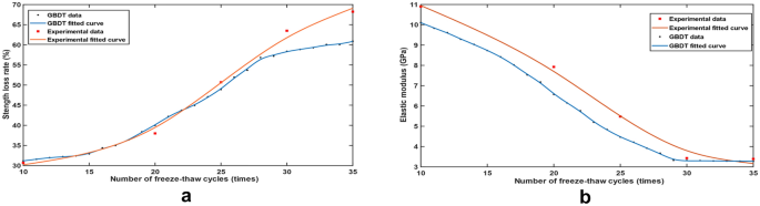
Fitted curves of experimental data and the AMGBDT model when the number of freeze–thaw cycles is adopted as a variable: a relationship between the strength loss rate and the number of freeze–thaw cycles; b relationship between the elastic modulus and the number of freeze–thaw cycles
-
(b)
The elastic modulus. Similarly, the two predicted curves have the same pattern of variation, with the elasticity modulus showing a decreasing trend with the increase of the number of freeze–thaw cycles. However, the magnitude of the change in the AMGBDT model fitted curve is slightly smaller than the experimental. In addition, the experimental curve fit's effectiveness is reduced due to the discrete nature of the experimental data points. The robustness of the AMGBDT model to missing values makes the dispersion of data points have less impact on the fitting effect.

The variation law of the fitted curve of the GBDT algorithm is basically the same as that of the fitted curve of the test. However, since the number of freeze–thaw cycles is set as the independent variable in the AMGBDT model only, the law of the number of freeze–thaw cycles and the decay of mechanical indexes obtained by the AMGBDT model is more accurate.
The influence of the initial porosity
The initial porosity is an inherent parameter of the rock, whose extent of influence in freeze–thaw cycles cannot be determined by experimental means. In other words, it is hard to obtain the experimental fitted curve of initial porosity and deterioration of mechanical properties. In the AMGBDT model, the number of freeze–thaw cycles as a fixed value, the strength decay rate is positively correlated with initial porosity, and the modulus of elasticity is negatively correlated with initial porosity. According to the magnitude of the curve, the deterioration caused by initial porosity as a variable is less than that caused by the number of freeze–thaw cycles. It was demonstrated that the number of freeze–thaw cycles had a more significant effect on the uniaxial compressive strength decay rate and elastic modulus than initial porosity. Figure 5 provides the exact changes in elastic modulus and uniaxial compressive strength of the sandstone after freeze–thaw cycles when the initial porosity is used as the independent variable.

Fitted curves of experimental data and the AMGBDT model when the initial porosity is adopted as a variable: a relationship between the strength loss rate and the number of freeze–thaw cycles; b relationship between the elastic modulus and the number of freeze–thaw cycles
Discussion
Different modeling methods can result in different impacts in mining the nonlinear mapping relationship between the independent vector X and the dependent vector Y. There are many studies on the application of GBDT in geological disciplines. In addition, RF, NN performs well in fitting highly nonlinear relationships. Therefore NN, RF, and the AMGBDT model are selected for fitting prediction.
The mutual constraints and interactions between neurons in the neural network algorithm enable the entire network to exhibit a nonlinear mapping from the input state space to the output state space. Therefore, the NN algorithm is suitable for solving problems with complex environmental information and unclear inference rules. The structure of the deep neural network used is shown in Fig. 6. The number of units in the input and output layers is 3 and 3, respectively, and the number of layers in the hidden layer is 3. The connection between layers is fully connected with each other. The number of neurons in each hidden layer is 128, 64, 32, respectively. Batch Normalization is used to solve the problem of gradient disappearance in deep neural networks, increasing the training speed of the network.

Structure of the NN
A random forest is composed of many decision trees in a randomly selected subset of training data [31], where each tree in the forest is voted on and decided jointly at decision time [32]. It performs well on a number of datasets and can handle high-dimensional data [33]. In addition, RF does not select features and can be computed in parallel to speed up training. RF exhibits some fault tolerance for training data and is an effective method for estimating missing data. Moreover, RF suits multi-classification problems and detects the interactions between variable features and the degree of importance. The number of trees in the random forest is 100.
Furthermore, the AMGBDT model's Score calculated by Eq. (10) is chosen as the evaluation index. The Score of the three models is shown in Fig. 7. A higher value of Score indicates a better prediction. The comparison in Fig. 7 illustrates that with the number of freeze–thaw cycles and initial porosity as independent variables, the Score value of the AMGBDT model is closer to 1 than the remaining two algorithms, which means that the AMGBDT fits best. Therefore, the AMGBDT algorithm with multiple outputs has been proven to be the most accurate.

Score of three methods
Conclusions
To study the effects of freeze–thaw cycles and initial porosity changes on the deterioration of mechanical properties of sandstone under freeze–thaw cycles, an AMGBDT model was developed for the study in this paper. Some limitations should be noted. The initial porosity is adopted as the independent variable when we explore the extent of influence of pore space inside the rock in the freeze–thaw damage. Due to the low cost and accessibility of the measurement of connected porosity and the considerable contribution in the freeze–thaw cycle deterioration, the initial porosity in this paper refers to the connected porosity. The frost damage mechanism of sandstone [34] demonstrates that both closed pores and connected pores contribute to rock freeze–thaw damage. The role of connected pores during freeze–thaw cycles may be amplified to some extent because no data on closed pores were measured in our study.
The conclusions are as follows.
-
(1)
Based on the theory of SQP and GBDT, the AMGBDT algorithm is proposed to allow its application to explore the effects of freeze–thaw cycling on the macroscopic deterioration patterns of sandstones in various locations.
-
(2)
The comparison of the prediction curves of the AMGBDT model with the curves fitted to the experimental data yields the following conclusions. When the initial porosity is fixed and the number of freeze–thaw cycles is the variable, the predicted curve of the AMGBDT model follows the same trend as the fitted curve of the test. However, the change in the decay rate of strength and elasticity modulus is less than the change range corresponding to the experimental curve. When the number of freeze–thaw cycles is fixed, and initial porosity is the variable, the changes in strength decay rate and modulus of elasticity are small and positively correlated. In summary, for dense rocks like sandstone, both initial porosity and the number of freeze–thaw cycles exacerbate the deterioration of mechanical properties, and the number of freeze–thaw cycles is the dominant factor.
-
(3)
The NN and RF are selected to perform the same training prediction. Comparing the Score of three models reveals that the model built by the AMGBDT algorithm performs optimally, which illustrates the feasibility of the proposed method.
The model constructed in this paper can be further applied to the multi-field coupling analysis of rock weathering to obtain the degree of contribution of the influencing factors of each action field to the deterioration of the final mechanical properties. The influence ranking weights of each factor at the time of coupling are obtained, and the mechanism of multi-field coupling can be further studied.
Availability of data and materials
Data sharing is not applicable to this article as no datasets were generated or analyzed during the current study.
Abbreviations
- AMGBDT:
-
An adaptive multi-output gradient boosting decision trees
- SQP:
-
Sequential quadratic programming
- NN:
-
Neural networks
- RF:
-
Random forests
- ML:
-
Machine learning
- CART:
-
Classification and regression trees
- SVM:
-
Support vector machine
- KNN:
-
K-nearest neighbor
- XGB:
-
Extreme gradient boosting
- LGB:
-
Light gradient boosting machine.
- \(D\) :
-
Data set of the freeze–thaw cycle experiment
- \(X\) :
-
Independent variables of the freeze–thaw cycle experiment data
- \(Y\) :
-
Dependent variable of the freeze–thaw cycle experiment data set
- \({ftt}_{i}\) :
-
Number of freeze–thaw cycles of the \(i\)th sample
- \({p}_{i}\) :
-
Porosity of the \(i\)th sample
- \({v}_{i}\) :
-
Longitudinal wave velocity of the \(i\) th sample
- \({sl}_{i}\) :
-
Loss rate of uniaxial compressive strength
- \({e}_{i}\) :
-
Elastic modulus after the deterioration of the \(i\)th sample
- \(m{l}_{i}\) :
-
Loss rate of mass
- \(N\) :
-
Number of samples
- \({F}_{0}\left({X}_{i}\right)\) :
-
Initial base regressor
- \(T\) :
-
Number of iterations
- \({b}_{ti}\) :
-
Negative gradient of the loss function in this iteration
- \(\mathcal{L}\left(\bullet \right)\) :
-
Loss function
- \({B}_{tj}\) :
-
The corresponding leaf node region of the regression tree
- \(J\) :
-
Number of leaf nodes of \(t\)th regression tree
- \({c}_{tj}\) :
-
The best-fit value for each leaf node region
- M :
-
Number of trees
- µ :
-
Learning rate of a model
- \(f\left({\varvec{Z}}\right)\) :
-
Objective function of the optimization problem
- \({{\varvec{Z}}}^{k}\) :
-
Current iteration point
- \(S\) :
-
Variable
- \({S}^{*}\) :
-
Optimum solution of the current problem
- \({S}^{k}\) :
-
The next search direction
- \({{\varvec{Z}}}^{k+1}\) :
-
An approximate solution to the original problem
- \(Score\) :
-
Coefficient of determination
- \({X}_{ik}\) :
-
Independent variable
- \({{X}_{ik}}^{^{\prime}}\) :
-
Independent variable after normalization
References
Wang JH, Yan SJ, Ren WZ, Fang Y. Research on structural stability analysis and evaluation system of cave rock body. Wuhan: China University of Geosciences Press; 2013.
Ke B, Zhou KP, Xu CS, Deng HW, Li JL, Bin F. Dynamic mechanical property deterioration model of sandstone caused by freeze-thaw weathering. Rock Mech Rock Eng. 2018;51(9):2791–804. https://doi.org/10.1007/s00603-018-1495-0.
Zhang J, Deng HW, Taheri A, Ke B, Liu CJ, Yang X. Degradation of physical and mechanical properties of sandstone subjected to freeze-thaw cycles and chemical erosion. Cold Regions Sci Technol. 2018;155:37–46. https://doi.org/10.1016/j.coldregions.2018.07.007.
Inada Y, Kinoshita N, Ebisawa A, Gomi S. Strength and deformation characteristics of rocks after undergoing thermal hysteresis of high and low temperatures. Int J Rock Mech Mining Scie Geomech. 1997;34(3–4):688. https://doi.org/10.1016/S1365-1609(97)00048-8.
Yahaghi J, Liu HY, Chan A, Fukuda D. Experimental and numerical studies on failure behaviours of sandstones subject to freeze-thaw cycles. Transportation Geotech. 2021;31:100655. https://doi.org/10.1016/j.trgeo.2021.100655.
Xu JC, Pu H, Sha ZH. Mechanical behavior and decay model of the sandstone in Urumqi under coupling of freeze-thaw and dynamic loading. Bull Eng Geol Environ. 2021;80(4):2963–78. https://doi.org/10.1007/s10064-021-02133-5.
Gao F, Xiong X, Zhou KP, Li JL, Shi WC. Strength deterioration model of saturated sandstone under freeze-thaw cycles. Rock Soil Mech. 2019;40(3):926–32. https://doi.org/10.16285/j.rsm.2017.1886.
Huang SB, Ye YH, Cui XZ, Cheng AP, Liu GF. Theoretical and experimental study of the frost heaving characteristics of the saturated sandstone under low temperature. Cold Regions Sci Technol. 2020;174:103036. https://doi.org/10.1016/j.coldregions.2020.103036.
Sarici DE, Ozdemir E. Determining point load strength loss from porosity, Schmidt hardness, and weight of some sedimentary rocks under freeze-thaw conditions. Environ Earth Sci. 2018;77(3):1–9. https://doi.org/10.1007/s12665-018-7241-9.
Li JL, Zhou KP, Liu WJ, Deng H. NMR research on deterioration characteristics of microscopic structure of sandstones in freeze–thaw cycles. Trans Nonferrous Metals Soc China. 2016;26(11):2997–3003. https://doi.org/10.1016/S1003-6326(16)64430-8.
Yu J, Chen X, Li H, Zhou JW, Cai YY. Effect of freeze-thaw cycles on mechanical properties and permeability of red sandstone under triaxial compression. J Mountain Sci. 2015;12(2):218–31. https://doi.org/10.1007/s11629-013-2946-4.
Jakubowski J, Stypulkowski JB, Bernardeau FG. Multivariate Linear Regression and CART Regression Analysis of TBM Performance at Abu Hamour Phase-I Tunnel. Arch Min Sci. 2017;62(4):825–41. https://doi.org/10.1515/amsc-2017-0057.
Armaghani DJ, Asteris PG, Askarian B, Hasanipanah M, Tarinejad R, van Huynh V. Examining hybrid and single SVM models with different kernels to predict rock brittleness. Sustainability. 2020;12(6):1–17. https://doi.org/10.3390/su12062229.
Yao BZ, Yang CY, Yao JB, Sun J. Tunnel surrounding rock displacement prediction using support vector machine. Int J Comput Intell Syst. 2010;3(6):843–52. https://doi.org/10.1080/18756891.2010.9727746.
Gupta S, Mohan N, Kumar M. A Study on Source Device Attribution Using Still Images. Arch Comput Methods Eng. 2021;28(4):2209–23. https://doi.org/10.1007/s11831-020-09452-y.
Akbulut Y, Sengur A, Guo YH, Smarandache F. NS-k-NN: Neutrosophic set-based k-nearest neighbors classifier. Symmetry. 2017;9(9):1–10. https://doi.org/10.3390/sym9090179.
Bansal M, Kumar M, Kumar M, Kumar K. An efficient technique for object recognition using Shi-Tomasi corner detection algorithm. Soft Comput. 2021;25(6):4423–32. https://doi.org/10.1007/s00500-020-05453-y.
Breiman L. Statistical modeling: The two cultures. Stat Sci. 2001;16(3):199–231. https://doi.org/10.1214/ss/1009213726.
Zhang Y, Haghani A. A gradient boosting method to improve travel time prediction. Transport Res. 2015;58:308–24. https://doi.org/10.1016/j.trc.2015.02.019.
Breiman L. Bagging Predictors. Mach Learn. 1996;24:123–40. https://doi.org/10.1023/A:1018054314350.
Wang YY, Wang DJ, Geng N, Wang YZ, Yin YQ, Jin YC. Stacking-based ensemble learning of decision trees for interpretable prostate cancer detection. Applied Soft Computing J. 2019;77:188–204. https://doi.org/10.1016/j.asoc.2019.01.015.
Freund Y, Robert E, Schapire. A short introduction to boosting. J Jpn Soc Artif Intell 1999;14(5):771–80.
Kuncheva LI, Bezdek JC, Duin RPW. Decision templates for multiple classifier fusion: an experimental comparison. Pattern Recogn. 2001;34(2):299–314. https://doi.org/10.1016/S0031-3203(99)00223-X.
Elith J, Leathwick JR, Hastie T. A working guide to boosted regression trees. J Anim Ecol. 2008;77(4):802–13. https://doi.org/10.1111/j.1365-2656.2008.01390.x.
Wang Y, Feng LW, Li SJ, Ren F, Du QY. A hybrid model considering spatial heterogeneity for landslide susceptibility mapping in Zhejiang Province, China. CATENA. 2020;188:104425. https://doi.org/10.1016/j.catena.2019.104425.
Liu JJ, Liu JC. An intelligent approach for reservoir quality evaluation in tight sandstone reservoir using gradient boosting decision tree algorithm - A case study of the Yanchang Formation, mid-eastern Ordos Basin, China. Marine and Petroleum Geology. 2021;126:104939. https://doi.org/10.1016/j.marpetgeo.2021.104939
Chen T, Zhu L, Niu R, Trinder CJ, Peng L, Lei T. Mapping landslide susceptibility at the Three Gorges Reservoir, China, using gradient boosting decision tree, random forest and information value models. J Mountain Sci. 2020;17(3):670–85. https://doi.org/10.1007/s11629-019-5839-3.
Friedman JH. Greedy function approximation: a gradient boosting machine. Ann Stat. 2001;29(5):1189–1232. http://www.jstor.org/stable/2699986
Radosavljević J, Jevtić M. Hybrid GSA-SQP algorithm for optimal coordination of directional overcurrent relays. IET Gener Transm Distrib. 2016;10(8):1928–37. https://doi.org/10.1049/iet-gtd.2015.1223.
Boggs PT, Tolle JW. Sequential quadratic programming. Acta Numer. 1995;4:1–51. https://doi.org/10.1017/S0962492900002518.
Kumar M, Jindal MK, Sharma RK, Jindal SR. Performance evaluation of classifiers for the recognition of offline handwritten Gurmukhi characters and numerals: a study. Artif Intell Rev. 2020;53(3):2075–97. https://doi.org/10.1007/s10462-019-09727-2.
Breiman L. Random Forests. Mach Learn. 2001;45:5–32. https://doi.org/10.1023/A:1010933404324.
Bansal M, Kumar M, Kumar M. 2D Object Recognition Techniques: State-of-the-Art Work. Arch Comput Methods Eng. 2021;28(3):1147–61. https://doi.org/10.1007/s11831-020-09409-1.
Jia HL, Ding S, Zi F, Dong YH, Shen YJ. Evolution in sandstone pore structures with freeze-thaw cycling and interpretation of damage mechanisms in saturated porous rocks. CATENA. 2020;195:104915. https://doi.org/10.1016/j.catena.2020.104915.
Acknowledgements
Not applicable.
Funding
This research was not supported by any public funding.
Author information
Authors and Affiliations
Contributions
CCL completed the conceptualization, investigation, and original draft writing. YBL completed the methodology and formal analysis. WZR and JXW supervised the draft. WHX and SMC performed the investigation, data curation, and validation. All authors read and approved the final manuscript.
Corresponding author
Ethics declarations
Competing interests
The authors declare that they have no competing interests.
Additional information
Publisher's Note
Springer Nature remains neutral with regard to jurisdictional claims in published maps and institutional affiliations.
Rights and permissions
Open Access This article is licensed under a Creative Commons Attribution 4.0 International License, which permits use, sharing, adaptation, distribution and reproduction in any medium or format, as long as you give appropriate credit to the original author(s) and the source, provide a link to the Creative Commons licence, and indicate if changes were made. The images or other third party material in this article are included in the article's Creative Commons licence, unless indicated otherwise in a credit line to the material. If material is not included in the article's Creative Commons licence and your intended use is not permitted by statutory regulation or exceeds the permitted use, you will need to obtain permission directly from the copyright holder. To view a copy of this licence, visit http://creativecommons.org/licenses/by/4.0/. The Creative Commons Public Domain Dedication waiver (http://creativecommons.org/publicdomain/zero/1.0/) applies to the data made available in this article, unless otherwise stated in a credit line to the data.
About this article

Cite this article
Liu, C., Liu, Y., Ren, W. et al. An adaptive prediction method for mechanical properties deterioration of sandstone under freeze–thaw cycles: a case study of Yungang Grottoes. Herit Sci 9, 154 (2021). https://doi.org/10.1186/s40494-021-00628-8
Received:
Accepted:
Published:
DOI: https://doi.org/10.1186/s40494-021-00628-8