Fast adaptive multimodal feature registration (FAMFR): an effective high-resolution point clouds registration workflow for cultural heritage interiors

Abstract

Accurate registration of 3D scans is crucial in creating precise and detailed 3D models for various applications in cultural heritage. The dataset used in this study comprised numerous point clouds collected from different rooms in the Museum of King Jan III’s Palace in Warsaw using a structured light scanner. Point clouds from three relatively small rooms at Wilanow Palace: The King’s Chinese Cabinet, The King’s Wardrobe, and The Queen’s Antecabinet exhibit intricate geometric and decorative surfaces with diverse colour and reflective properties. As a result, creating a high-resolution full 3D model require a complex and time-consuming registration process. This process often consists of several steps: data preparation, registering point clouds, final relaxation, and evaluation of the resulting model. Registering two-point clouds is the most fundamental part of this process; therefore, an effective registration workflow capable of precisely registering two-point clouds representing various cultural heritage interiors is proposed in this paper. Fast Adaptive Multimodal Feature Registration (FAMFR) workflow is based on two different handcrafted features, utilising the colour and shape of the object to accurately register point clouds with extensive surface geometry details or geometrically deficient but with rich colour decorations. Furthermore, this work emphasises the challenges associated with high-resolution point clouds registration, providing an overview of various registration techniques ranging from feature-based classic approaches to new ones based on deep learning. A comparison shows that the algorithm explicitly created for this data achieved much better results than traditional feature-based or deep learning methods by at least 35%.

Introduction

The cultural heritage (CH) preservation field is currently experiencing a growing demand for high-resolution and high-quality 3D data in the form of point clouds. Precision 3D scanning is essential for accurately documenting the present state of an object’s preservation [1]. One can infer the CH object’s condition by analysing the acquired scan data. By conducting repeated scans over time, it is possible to track and document changes in the object’s state of preservation [2, 3]. Additionally, CH objects are exposed to different factors that cause their deterioration and degradation over time due to human activities and environmental factors. To protect and maintain cultural heritage objects and sites, it is essential to conduct architectural documentation, which involves creating 3D point clouds, 3D models, orthoimages, and vector drawings [4]. Such documentation enables a comprehensive and detailed understanding of the object or site and is crucial for preservation and restoration efforts. By generating accurate and precise digital representations of CH objects, documentation provides a valuable resource for research, education, and public awareness [5,6,7]. While many methods are available for digitising CH objects, such as 3D scanning or close-range photogrammetry, high-quality 3D point clouds are often necessary to record the intricate details of these objects accurately [8,9,10].

However, registering multiple 3D point clouds to create a complete digital representation of cultural heritage objects can be challenging, requiring a highly skilled operator and specialised tools. There are multiple registration methods available, each suited to different types of point cloud data acquired from various sources, such as 3D scanners [11], close-range photogrammetry [12], LiDAR (Light Detection and Ranging [13]), and structured light (SL [14]). These different point cloud data sources may have varying characteristics, such as point density, noise, and accuracy. In addition to the scanning technique, the different cultural heritage objects can also exhibit variations in surface parameters such as geometric details and colour. To handle the diversity in point cloud characteristics arising from different scanning techniques and surface properties, specific registration methods must be employed to ensure the accurate alignment of the 3D data. Therefore, it is crucial to evaluate the available registration methods [15] and select the one that best suits the specific needs of the particular CH documentation project. The salient point-based methods have mainly focused on searching for key points and calculating descriptors to match different point clouds of the same objects [16]. Neural network-based methods [17] have emerged as a promising alternative, but their effectiveness has primarily been demonstrated in industry, where objects are more uniform, homogenous, and repetitive [18, 19]. Despite their effectiveness in industrial settings, these methods are not always suitable for registering CH objects due to the unique nature of each manifested difference in geometry, surface, or colour. Additionally, the learning process for these methods can be lengthy, and training sets for cultural heritage objects are often not readily available, making their use impractical in many cases. Moreover, due to the uniqueness of their surfaces, it is challenging to prepare a proper training set which could be adapted to supervised learning.

To conclude, the previously mentioned point cloud registration methods can be divided into two main categories: pairwise and multiview registration [20]. The selection of the appropriate method depends on the number of point clouds to be processed. Utilising multiview registration methods requires determining approximate point cloud orientation parameters and knowing the order of the processed point clouds. For this reason, the quality of determining the relative orientation between the point clouds affects the accuracy of the final bundle adjustment.

Data in this study consist of a substantial amount of point clouds, captured by a structured light scanner, from various rooms in the Museum of King Jan III’s Palace in Warsaw. Those measurements produced high-resolution architectural documentation in the form of point clouds with a resolution of 100 points per square millimetre. This high resolution was necessary to analyze micro-scale degradation and shape changes accurately. Additionally, these requirements and resolutions were driven by the needs of the museum’s conservators. The structured light (SL) method was chosen because it can accurately map the object’s shape and colour. The surfaces of the point clouds used in this study are rich geometrically and decorative through surface colour and different reflective properties. As a result, multiple registration methods with varying parameters would be necessary, requiring extensive and time-consuming work by skilled operators to align all point clouds into a single 3D model, totalling approximately 14 billion measurement points. Given these considerations, there is an apparent necessity to develop an efficient and fast workflow for registering point clouds in this case.

This study aimed to propose a novel pairwise workflow, named Fast Adaptive Multimodal Feature Registration (FAMFR), used for highly accurate point cloud registration for CH object’s interiors. The proposed FAMFR workflow is based on two steps: (1) initial point cloud registration relying on local geometry and colour at each point of the point cloud and (2) final pairwise registration. To detect tie points (initial registration), two approaches were developed: one based on the histograms of RGB intensity gradients and the other based on the relation between normal vectors in a local neighbourhood, similar to the point pair feature (PPF [16]). The final pairwise registration is completed by using a modified commonly used ICP (Iterative Closest Point [21, 22]) method based on the selection of correspondent points based on a texture/colour similarity metric. The obtained pairwise registration results are used, in a further step, by the final bundle adjustment of the multiple-point clouds.

The research follows a structured approach with a literature review of Related works, followed by Materials which describe the datasets used in the study. The Methods section then presents the algorithms, schemes, and overall workflow used to register point clouds of CH objects. The Results and Discussion sections present and comment on a comparative analysis of various state-of-the-art methods and registration outcomes. The paper concludes with a summary of the findings, critical analysis, and future directions for similar research.

Related works

The increasing availability of various sensors and methods for CH documentation, namely: ultra-light Unmanned Aerial Vehicles (UAVs) [23], devices such as laser scanners or triangulation scanners [24], mobile phones with built-in LiDAR sensors [25], and close-range photogrammetry software [26] facilitated the generation of point clouds with much wider dissemination than in previous decades. This has led to more documentation projects in the cultural heritage domain as the ease of obtaining point clouds has improved. Non-professionals can contribute to CH documentation, preservation, and restoration efforts by capturing and sharing high-quality point clouds of heritage sites. This has enabled a more comprehensive range of people to engage in the process of digitally documenting and preserving CH. As a result, it has become easier to identify, study, and restore important cultural heritage sites, leading to a greater understanding and appreciation of our shared history and culture.

Fig. 1

Visualisation of the point clouds registration process

3D point clouds have become an essential data source for digitisation in the CH field. They are widely used for tasks such as Historical Building Modelling (HBIM), Structural Health Monitoring (SHM), damage detection, documentation, and virtual restoration [27]. Point clouds can accurately represent the geometry and colour of the object’s surface, making them a valuable tool for documenting and preserving CH objects. Point clouds are employed for a wide range of tasks, including segmentation [28], classification [29], 3D documentation [30], and modelling applications [31]. For most cultural heritage objects’ 3D documentation, an additional task, such as registration, is required to produce a complete representation. This is especially true for objects that require multiple point clouds to depict a complete structure, terrain, or CH complex surface. Obtaining data from a single 3D scanner position is impractical for large CH objects and sites, and multiple point clouds need to be registered into one 3D representation. It is done by aligning multiple point clouds into a common coordinate system. It is done by finding and applying the best 3D transformation between them; see Fig. 1.

Consequently, numerous registration methods have been developed to address this issue. Some examples include registering TLS (Terrestrial Laser Scanning) point clouds using two ICP variations [32], constant radius features for large scale and detailed CH object registration [33], automatic registration of overlapping point clouds using external information acquired from corresponding images [34] or employing feature-based methods [35]. These workflows are designed to register and combine multiple point clouds into a comprehensive and accurate representation of the object or site of interest. Usually, the registration process is divided into two stages. The first involves an initial matching step, where point clouds are roughly aligned. The second stage utilises the iterative closest point algorithm for fine matching, which can accurately tune the initial 3D transformation between the point clouds (Fig. 2). There is plenty of variants of ICP algorithms which are widely used in point cloud alignment workflows. The ICP algorithm is dependent on accurate enough initial matching.

Fig. 2

Two-stage registration process; a input pair cloud, b initial registration, c fine registration and d final model

One of the main challenges in point cloud registration for CH objects is the vast differences in shape, texture, colour, rich decorations, and varying state of preservation. These objects were created in various historical periods and stored under different conditions. Additionally, occlusions and measurement noise are unavoidable in point clouds and can affect the final model. Varying lighting conditions and partially reflective and transparent surfaces can lead to some colour and geometry reconstruction imperfections, adding errors during point cloud registration workflows [36].

Point cloud registration techniques can be categorised into three main groups: feature-based (hand-crafted), iterative, and deep learning. Each category can be further classified based on whether they use geometric information, colour information, or both see Fig. 3.

Fig. 3

Registration method classification

Choosing the correct registration method is crucial to handle differences between point clouds because geometry-based methods may only be suitable for scans with extensive surface geometry details. In contrast, clouds that lack geometric details necessitate the analysis of texture/colour information for precise registration. Therefore, the object’s colour and shape must be considered. Overlapping regions in data can also pose challenges, especially when the overlapping region of processed point clouds is too small for the used method to handle effectively. Finally, a photogrammetric network can achieve good registration results based on the marked control points [37]. However, that method is not suitable for CH objects because, in most cases, it is impossible to distribute those points on the object’s surface. The solution to this disadvantage may be using a feature-based registration approach based on automatically detected key points, also known as local features.

The registration workflow based on local features is a multi-step process that involves key point detection [38], descriptor calculation [39], correspondence calculation based on the descriptor matching approach and geometrical verification that allows obtaining reliable tie points [40]. The feature-based methods extract 3D key points from the object’s surface—reliable and stable points for effective description and matching. There are many algorithms for detecting these features, and among the most commonly used we can include SIFT (Scale-invariant feature transform [41, 42]), SURF (Speeded up robust features [43, 44]), ISS (Intrinsic Shape Signatures [45]), and Harris3D [46]. Based on local or global neighbourhoods, the point descriptors assign characteristic values (changes in grey degree gradients, colour or shape) to the detected key point. The algorithms used to calculate descriptors vary in execution time and accuracy, and their effectiveness depends on the character of input 3D data. Some rely on the geometry of the object’s surface, some on colour, and some on both features simultaneously [47]. The popular descriptors, namely: Point Pair Feature Histograms (FPFH) [48], Spin Images [49], and Signature of Histograms of OrienTations (SHOT) [50], are used for describing the local features and further used for the finding correspondence points in matching step. The point clouds’ key points and descriptors can be initially integrated based on the 6-degree of freedom transformation and RANSAC [51] searching correspondence phase. After that step, the ICP algorithm allows for achieving fine registration results.

Another group of methods used in point clouds registration are those based on a deep learning-based approach, and with their development, accuracy and efficiency in this area has developed [52]. Furthermore, there is a rising trend in sharing publicly available datasets designed for machine learning applications in the CH field [53, 54]. One of the significant advancements in deep learning point cloud processing is PointNet [55] because it provides a unified architecture that can directly take point clouds as input. The basic architecture of PointNet is straightforward, where each point is processed independently and identically in the initial stages. The point is represented by its three coordinates (x, y, z), and other layers can be added by computing normal vectors or additional features. PointNetLK [56] adapts the Lucas and Kanade (LK) algorithm to work with PointNet and unrolls it into a single recurrent deep neural network. This allows for global feature alignment and demonstrates strong generalisation across shape categories while maintaining computational efficiency, but it is not robust to noise. In [57], authors propose a DeepGMR registration method that combines Gaussian Mixture Model (GMM) with neural networks to extract pose-invariant correspondences between raw point clouds and GMM parameters. This method estimates the correspondence between all points and all components in the latent Gaussian Mixture Model (GMM). It performs well across challenging scenarios, such as noise and unseen geometry. The DCP (Deep Closest Point [58]) is an algorithm that utilises a DGCNN (Dynamic Graph Convolutional Neural Network [59]) network to learn correspondences and a differentiable Single Value Decomposition (SVD) method for registration. It encodes point clouds into a high-dimensional space using PointNet or DGCNN and uses an attention-based module to capture contextual information. The method employs a differentiable SVD layer to estimate the alignment. The DCP has shown promising results on shapes not encountered during training. However, this method assumes an exact one-to-one correspondence between the two point cloud distributions, which may not always hold in real-world scenarios where point clouds may be subject to outliers and other uncertainties, and its performance is hindered by noise. Many state-of-the-art deep learning registration methods rely solely on geometry information, neglecting texture information. However, some exceptions exist where these methods rely on intermediate media such as RGBD images, projection images, or depth maps [60,61,62]. Since deep learning methods typically process only relative positions of points, they lack colour information, which limits their applications. Texture information enables humans to distinguish different parts of a scene. In the context of CH, objects of interest often feature intricate details and rich ornamentation that may have different colours and textures. Therefore, incorporating colour information in point cloud registration can produce more reliable and accurate results. In addition, deep learning methods for CH point cloud registration face certain limitations, such as the requirement for substantial training data and the possibility of overfitting. Furthermore, the current point descriptors based on deep learning are often considered black boxes, lacking a clear understanding of how the original points are processed to generate the final descriptor.

Materials

Cultural heritage site

The Wilanów Palace is the only Baroque royal residence in Poland. Construction of this summer residence began at the end of the 17th century and has been repeatedly expanded and modernised. The palace’s two-story building hides many relatively small rooms but is characterised by a rich and varied interior design. This makes visiting the residence attractive, and another surprise awaits the visitor behind every corner of the palace corridor. However, this situation also creates severe challenges for the museum. Creating a program of precise three-dimensional documentation of selected interiors is one attempt to deal with these problems. The complex interior layout of the palace complicates providing visitors with access to all rooms. Due to conservation restrictions and security considerations, some rooms can only be accessed by tourists by looking inside through open doors, and sometimes even this form of access is impossible. Creating and providing high-quality digital documentation ensures these magnificent interiors can function in the public domain. Another problem arises from the fact that the Palace, built as a summer residence and characterised by thin walls, now functions as an all-year museum in the harsh conditions of the Polish climate. The inability to lay adequate thermal insulation makes it a significant challenge to ensure appropriate environmental conditions in the palace’s interiors at different times of the year. Monitoring the state of preservation of the wall paintings, wooden polychrome ornaments, and other elements of the interior design is an easier task when one has precise spatial documentation that gives the possibility of verifying even minor changes.

The King’s Chinese Cabinet and the King’s Wardrobe are two rooms in the southern part of the palace used by the King. The third of the rooms that are the subject of this article is the Queen’s Antecabinet, located on the other northern side of the palace’s central axis and in part used by the Queen. All three rooms have similar dimensions of 4[m] by 4[m] and a height of 5[m] (Fig.  4).

Fig. 4

The floor plan of the palace interiors. Red squares mark the rooms used in this study [63]

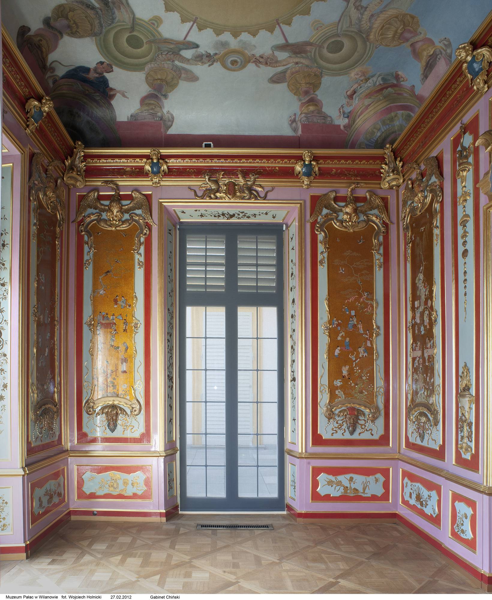
The current decoration of the King’s Chinese Cabinet (see Fig. 5) is the work of the workshop of Martin Schnell, who was court lacquerer and painter to King August II the Strong. The wall decoration, created around 1730, is in the form of polychrome wooden panels painted with lacquer and then covered with tiny pieces of silvered copper, which gives the decoration its characteristic glare. The ceiling is covered with a wall painting that relates in theme and colour to the wall decoration but is characterised by much less glare.

Fig. 5

The King’s Chinese Cabinet [64]

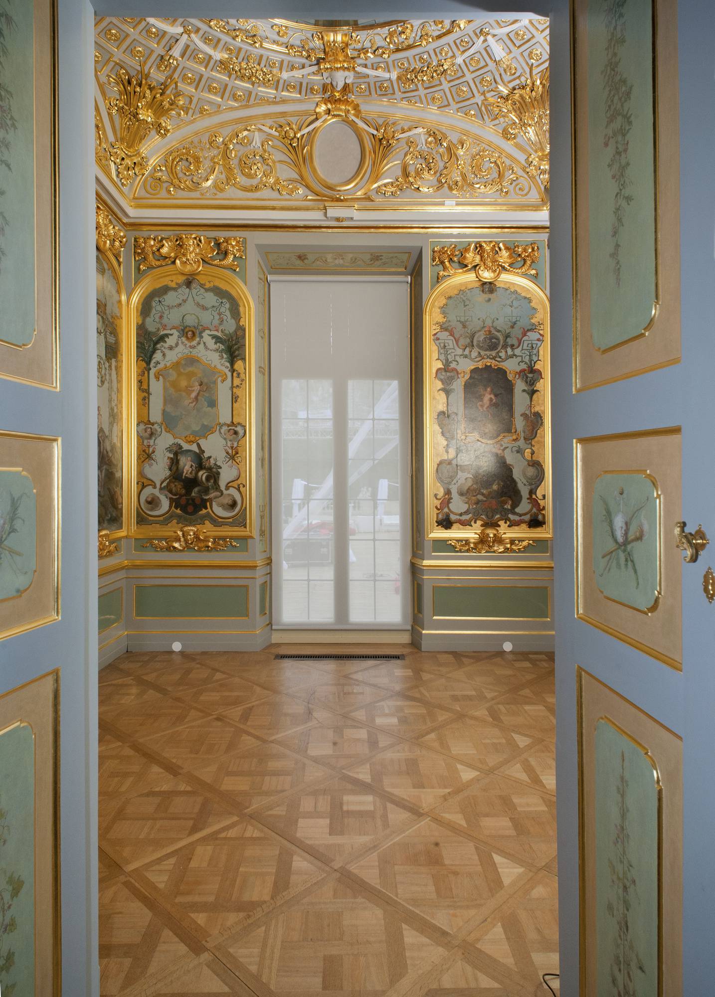
From the King’s Chinese Cabinet, it is possible to enter the King’s Wardrobe (Fig. 6), which has ceiling decoration dating back to the time of King John III and wall decoration made after 1730. Here, too, the walls are covered with wooden panels, into which paintings were created by a group of Saxon artists, who emphasise in their subject matter the connection between the interior of the palace and the surrounding nature of the gardens. The decoration of this room is dominated by light colours combined with a large number of gilded surfaces.

Fig. 6

The King’s Wardrobe [65]

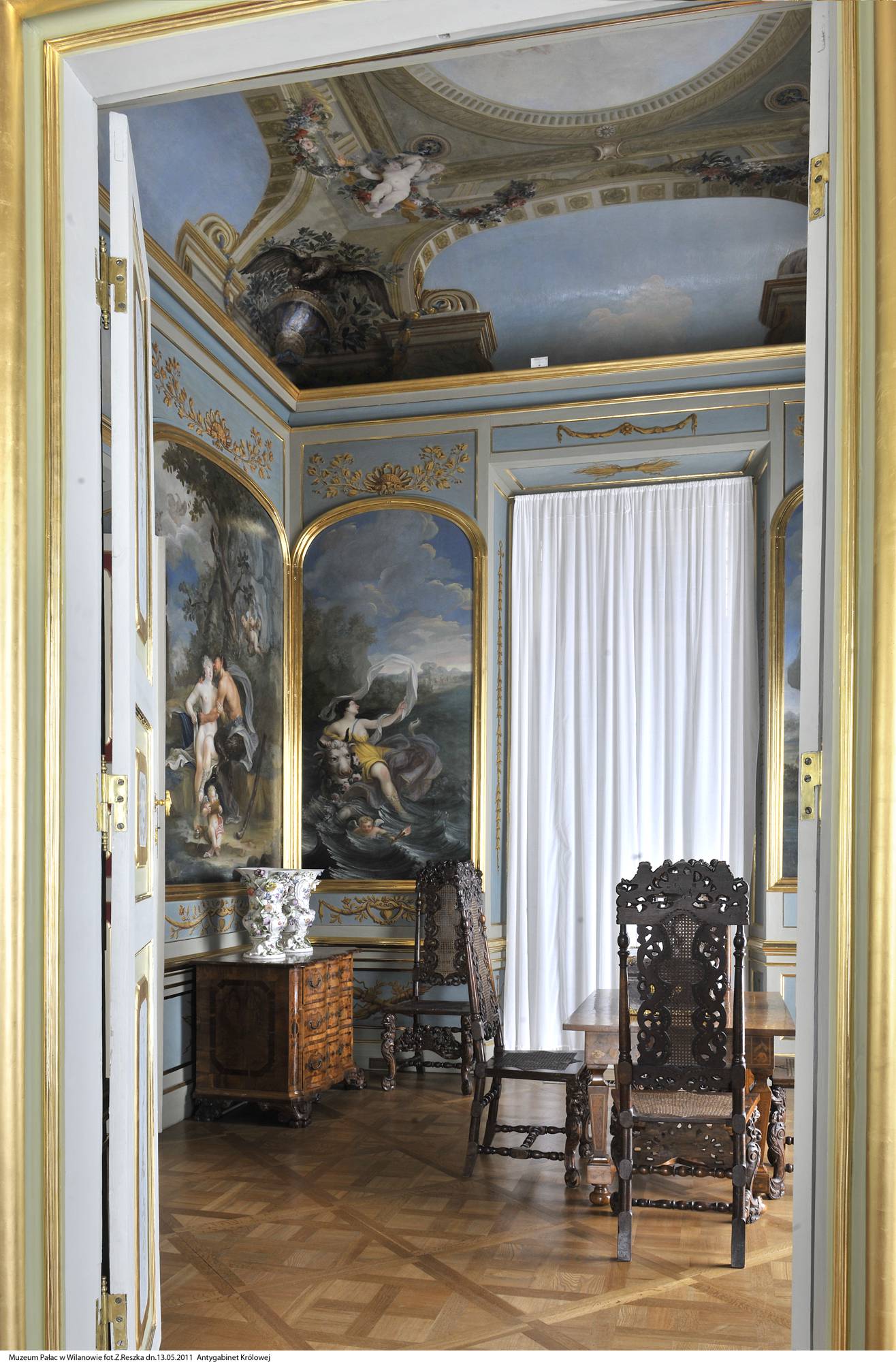
The Queen’s Antecabinet (see Fig. 7), whose decoration is dated to 1732, when the Wilanów Palace was used by King August II the Strong. The illusionistic Plafond painting in this room is the work of Jules Poison. The walls are decorated with scenes alluding to Greek mythology, as described by Ovid in his work “Metamorphoses”. Thus, we are dealing with wooden wall coverings and inserted panels with oil painting.

Fig. 7

The Queen’s Antecabinet [66]

Acquisition system

Single 3D point clouds were captured by a custom measurement system designed for the interior acquisition campaign [67], see Fig. 8. The system was designed to emphasise partial acquisition automation [68, 69], thus achieving high-quality measurement data regarding resolution, accuracy, and colour. The high resolution was crucial for analysing cracks, scratches, and other imperfections in specific object parts.

The structured light 3D scanner has a specially designed LED projector and two detectors for shape and colour acquisition. The digital projector has a native resolution of 1280 $\times$ 800 pixels and is used for the projection of the fringes onto the object’s surface. The spectral properties of the custom LED light sources have been reviewed and approved by the Conservation Department of the Museum. To ensure wider coverage of the surface being measured, two Point Grey colour cameras with a resolution of 9 megapixels each are mounted on the left and right sides of the projector.

A 3D scanner was mounted on an industrial robot arm to support partial automation of measurements. The colour was captured using six images with different directions of light illumination to remove the specular component. Two illuminators were mounted on the measurement head and four on the robot base. The robot arm was mounted on a vertical lift, capable of reaching up to 5.5[m]. The system was based on a stabilised platform with trolley wheels for easy movement.

Fig. 8

Measurement system

Data

The number of point clouds captured during a single room 3D digitisation is massive (around five thousand for each room). Each point cloud contains approximately 7.5 million points (see Fig.  9). The geometrical uncertainty of the point clouds is lower than 0.05 [mm], with an average point-to-point distance of 0.1 [mm]. Every point in the point cloud is represented by its 3D coordinates, normal vector, and calibrated colour values (R, G, B).

Fig. 9

Point cloud examples in comparison to the entire King’s Chinese Cabinet room

The dataset used in this paper is a subset of the captured cloud of points, and it has been divided into four subcategories (Fig. 10). The first one comprises point clouds with high-detailed geometry that accurately represents the surface shape (Fig. 10c). The second one consists of planar point clouds characterised by various colours, primarily representing paintings and artworks (Fig. 10d). The third subcategory combines the previous two characteristics, featuring decorative paintings on curved ceilings (Fig. 10a), and the final most challenging subcategory comprises a room fragment containing numerous gilded and shiny decorations (Fig. 10b). However, it should be emphasised that high levels of measurement noise distinguish point clouds belonging to the last subcategory. All data acquired by the scanner suffers from the specular reflections caused by light bouncing off shiny surfaces. Despite using six light sources during scanning, resulting point clouds still contain artefacts and noise due to this factor (Fig. 11).

Fig. 10

Four different point cloud examples: a ceiling point clouds, b shiny/glided point clouds, c point clouds with rich shape, d point clouds without shape variations

Fig. 11

Reflective surface point cloud artefacts

Method

Figure 12 presents an overview of the FAMFR workflow. To obtain an accurate final model, several algorithms were proposed and developed. Combining them enabled the accurate registration of the point clouds.

Fig. 12

FAMFR registration workflow

Preprocessing

To speed up the registration process without decreasing accuracy and reduce storage requirements, point clouds were uniformly sampled by a factor $N_{sim}$. This factor is equal to the ratio of the number of points before sampling to the number of points after sampling. After sampling, an average point-to-point distance $D_{avg}$ is calculated. It will be used as a parameter for subsequent algorithms. Next, two metrics were calculated for each point cloud, stable and transformed ($P_s$ and $P_t$): vector of point pair features $V_s$ and gradient of RGB intensities $I_g$. The first is calculated as follows: for each point, p, a neighbourhood sphere with a radius equal to $R_n \cdot D_{avg}$ in a cloud around the point of interest is created. Then, three angular values are calculated: $V_s(\alpha , \beta , \gamma )$. It is described by the distance between neighbouring points $p_n$ around p and the relative angles of normal vectors associated with those points n and $n_n$ according to Fig. 13 and formula 1.

Fig. 13

Point pair feature relations

$$\begin{aligned} \begin{aligned} V_s = (\angle (n,d), \angle (n_n,d), \angle (n,n_n)). \end{aligned} \end{aligned}$$

(1)

The intensity gradient $I_{g}$ at a given point p is a vector orthogonal to the normal vector n with the direction of the maximum gradient in the local intensity. The magnitude of the vector indicates the gradient of intensity change. The descriptor is constructed based on the local neighbourhood $p_n$: for each point p an RGB luminosity L is calculated using formula 2.

$$\begin{aligned} \begin{aligned} L = 0.299 \cdot red + 0.587 \cdot green + 0.114 \cdot blue. \end{aligned} \end{aligned}$$

(2)

The coefficients used in the formula (0.299, 0.587, 0.114) are based on the luminosity function, a mathematical model of the human eye’s sensitivity to different wavelengths of light [70]. An average coordinate $p_{avg}$ is calculated from all the points $p_n$ inside the sphere. The next step is determining the average luminosity $L_{avg}$ of all neighbouring points $p_n$. Then, luminosity difference $L_d$ is calculated between average value $L_{avg}$ and $L_n$ for each point $p_n$ (see formula 3).

$$\begin{aligned} \begin{aligned} L_{avg} = \dfrac{\Sigma L_n}{n} \\ L_d = L - L_{avg}. \end{aligned} \end{aligned}$$

(3)

Finally, each of the neighbouring points $p_n$ is modified according to the $p_{avg}$ coordinates using the formula 4.

$$\begin{aligned} \begin{aligned} p_n = p_n - p_{avg}. \end{aligned} \end{aligned}$$

(4)

The matrix A and vector b are created according to the sum of neighbouring points coordinates; see formula 5.

$$\begin{aligned} \begin{aligned} A&= \begin{bmatrix} \Sigma p_{nx} \cdot p_{nx} &{} \Sigma p_{nx} \cdot p_{ny} &{} \Sigma p_{nx} \cdot p_{nz}\\ \Sigma p_{nx} \cdot p_{ny} &{} \Sigma p_{ny} \cdot p_{ny} &{} \Sigma p_{ny} \cdot p_{nz}\\ \Sigma p_{nx} \cdot p_{nz} &{} \Sigma p_{ny} \cdot p_{nz} &{} \Sigma p_{nz} \cdot p_{nz} \end{bmatrix} \\ b&= \begin{bmatrix} \Sigma p_{nx} \cdot L_d&\Sigma p_{ny} \cdot L_d&\Sigma p_{nz} \cdot L_d \end{bmatrix} \\ x&= A^{-1} \cdot b. \end{aligned} \end{aligned}$$

(5)

Once constructed, the matrix undergoes QR decomposition using the Householder method [71]. As a result of decomposition, the vector x is obtained. The intensity gradient $I_{g}$ is formed from three values $I_{g}(L_x, L_y, L_z)$ according to the formula 6.

$$\begin{aligned} \begin{aligned} I_g = (Identity -n \cdot n^T) \cdot x, \end{aligned} \end{aligned}$$

(6)

where Identity denotes the identity matrix and n normal vector, visualization of those two metrics describing the colour and shape of the point cloud is presented in Fig. 14 in the form of vector magnitudes.

Fig. 14

Feature vectors magnitude: on top input clouds, in middle shape vector magnitude $|V_s|$, bottom shows gradient magnitude $|V_g|$

Key points evaluation

The two vectors mentioned in the previous subsection allow identifying key points for the rough registration of point clouds. At first, from $P_s$ and $P_t$ point clouds, two individual subsets, respectively $P_{ss}$ and $P_{ts}$, of evenly distributed points with equal distance $K_d$ between them are selected. Next, key points are filtered based on the previously calculated $|V_s|$ and $|V_g|$ values. Subsets of points $P_{ss}$ and $P_{ts}$ are filtered to retain only those whose value is greater than the threshold of $T_h$ of the maximum value of the magnitude vector from the entire point cloud ($max(|V_s|)$ or $max(|V_g|)$). As a result, the key points were classified into two distinct categories based on their potential for the registration process. The first category involves points used for registration utilising the point pair feature vector. The second category consists of points intended for registration using intensity gradients. The whole process is presented in Fig. 15.

Fig. 15

Key points evaluation process on the geometrical features (right) and gradient features (left). a input cloud, b evenly distributed subset of points, c all potential key points split into two categories, utilising geometrical or gradient features, d key points filtered using threshold $T_h$, e) Final key points used for registration

Feature histogram

A histogram of angular values ($\theta$) in a given neighbourhood is determined for each selected point from $P_{ss}$ and $P_{ts}$ subsets independently. The feature is generated from the neighbourhood by calculating the angles between the feature vector ($V_s$ or $V_g$) at each point $p_s$, and the vector formed by the characteristic point $p_s$ and its neighbouring points $p_{sn}$. This neighbourhood is formed as a sphere with user-defined radius parameters separately for shape $H_s$, and gradient $H_g$. These radii are represented as the multiplication of $D_{avg}$ value. The procedure is illustrated below through a Fig. 16 and a formula 7.

$$\begin{aligned} \begin{aligned} v_n = p_n - p \\ \theta = v_n \cdot cos(\dfrac{v_n \cdot V}{|v_n||V|}). \end{aligned} \end{aligned}$$

(7)

Fig. 16

Histogram angle value

All calculated angles are assigned to the corresponding bin in the histogram, which is pre-divided into a fixed number of cells $H_b$. If the calculated angle for a specific neighbouring point $p_{sn}$ is within the given cell boundaries, then it is increased by the value of the gradient divided by the distance from key point $p_{sn}$ ($d_s = |p_{sn} - p_s|$). Finally, after all the angles are allocated to their respective cells, the histogram is normalised using the number of neighbouring points. Figure 17 presents key point examples with calculated histograms.

Fig. 17

Four different key points with histogram examples

Correspondence evaluation

The obtained histograms are used for identifying corresponding key points pairs between two point clouds via similarity coefficient S. The similarity coefficient is defined using a formula 8, where $f_{p_s}(i)$ and $f_{p_t}(i)$ are values of histogram bins from stable $p_s$ and transformed $p_t$ key points.

$$\begin{aligned} \begin{aligned} S = \sqrt{\frac{\sum _{i=1}^{H_b}(f_{p_s}(i)-f_{p_t}(i))^2}{\sum _{i=1}^{H_b}(f_{p_s}(i)+f_{p_t}(i))^2}}. \end{aligned} \end{aligned}$$

(8)

A lower similarity coefficient score indicates a better match between the points. A fixed number of matched point pairs is selected with the lowest similarity values to filter out an initial set of matched point pairs. A user-defined parameter determines the number of selected point pairs $N_p$.

A rigid transformation between point clouds requires three different, non-collinear point pairs. From $N_p$ set, all possible triplets are formed. To remove correspondence outliers spatial consistency of the triplets was analysed. Each of those triplets goes through a filtering process based on user-defined triangle similarity parameter $T_s$. It is a geometric concept describing the relationship between two triangles of similar shapes and sizes. All triplets are also described by the combined similarity $C_s$ of all point pairs within them. This value is utilised to filter the final set of correspondences further.

For each formed triplet, a 3D transformation is computed and applied to the $P_t$ point cloud, and matching quality is evaluated. The registration quality depends on two error metrics: correspondences recall and the similarity between gradient or shape vectors. The first value eliminates incorrect transformations that lead to a small overlapping region after registering two point clouds using said transformation. A specific number of final triplets are selected based on the user-defined parameter $N_T$ and the lowest possible combined similarity error $C_s$.

In the next step, the local feature vectors based on each point pair’s shape or gradient vector in the final triplet’s set are compared to determine optimal correspondences. These correspondences are then utilised to estimate a rigid transformation using the Umeyama algorithm [72].

The final step involves using the ICP algorithm for fine registration. In the shape-based registration approach, the closest point based on distance is selected for each iteration of the algorithm, while in the gradient-based approach, the similarity coefficient between gradient vectors is used.

Experiment and results

The FAMFR workflow was tested using a computer with 64 GB RAM, Intel Core I7-8850H 2.60 GHz CPU, and NVIDIA GeForce Quadro P1000.

Parametrisation of control parameters

The proposed method incorporates a small set of control parameters (see Table 1), which are critical in determining the overall performance of the FAMFR workflow. These parameters are inherently intuitive and should be configured based on the specific characteristics of the data. A recommended approach for parameter selection is to experimentally evaluate them based on a representative subset of point clouds from the CH object. Subsequently, a comprehensive evaluation of the efficacy of the selected parameters should be conducted on a larger sample of data or the entire dataset to verify the generalisation capacity of the user-defined parameters. It is possible to make the parameters dependent on the average distance between points as was described above to make it more user-friendly and to generalise this method to be used in the future across varying datasets. This significantly improves the method’s accessibility and usability.

Table 1 Method control parameters

The first parameter, $H_b$ represents the number of histogram bins. The value has the least impact on the whole process, and its value was determined experimentally. The number of histogram cells used in this study equals 18.

The following parameter, the sampling factor ($N_{sim}$), strongly relates to the data the user wants to integrate. This parameter should be given a higher value for dense point clouds to avoid excessive computational time. When dealing with smaller point clouds, a higher simplification factor can lead to the loss of crucial details and characteristic features, thereby hindering the registration process. The value of this parameter used in this study was set to 25. It results in the average point cloud with approximately 300,000 points and an average distance between points $D_{avg} = 0.7$ [mm].

Parameter $R_n$ defines the radius value that forms a neighbouring sphere. This sphere is used to estimate two feature vectors for each point. The $R_n$ value influences the precision of the calculated features. Decreasing the value enhances the detection of fine details, affecting the accuracy of the final alignment of point clouds. A greater value allows for more effective determination of cloud fragments for key points detection. See Fig. 18 for different parameter value results. The parameter value was set to $R_n = 7$, $7 \cdot D_{avg} \approx 5$ [mm] during the experiment.

Fig. 18

Data visualisation for different $R_n$ parameter values

Accurately identifying correspondences is the key aspect of the process, as it determines the initial registration of point clouds. Therefore, the main focus should be selecting the parameters responsible for this stage. The main parameter is the point-to-point distance $K_d$ used to select the subset of points. Setting this value too low substantially increases the time required for determining correspondences. The number of potential key points increases, thus the number of calculations needed to evaluate the histograms and their subsequent comparison. It takes around 266 [s] to initially evaluate correspondences from histograms for point clouds used in this study and $K_d = 2$. Although the number of correct correspondences, in that case, is very high and equals 455. See Fig. 19. The value was set to $K_d = 7$, $7 \cdot D_{avg} \approx 5$ [mm] throughout the experiment.

Fig. 19

Relation between parameter, time and correspondences found. The time axis is on a logarithmic scale

On the other hand, excessively high values of this parameter may result in selecting points that lack descriptive features and are not sufficiently unique to identify a correct match. In addition, the number of outliers (red lines in the Fig. 20) drastically increases.

Fig. 20

Correspondences result for different values of $K_d$ parameter

Another parameter closely related to key point estimation is $T_h$. It helps eliminate outliers and points that do not contribute enough shape or colour information to the registration process. A lower value of $T_h$ may result in selecting key points with insufficient and not unique feature values, which could introduce false positives in the point cloud registration. On the other hand, a high $T_h$ value may eliminate potentially correct correspondences, leading to a decrease in the accuracy of the registration workflow. $T_h$ value was set experimentally to 0.2 in this study.

The radius parameters $H_s$/$H_g$ are crucial in establishing correct correspondences between point clouds. Their values significantly influence the descriptiveness of the selected key points. In addition, higher radius values are related to higher processing times. Nonetheless, setting too high or too low values can elevate the number of outliers and hinder the registration process. Thus, a trial-and-error approach on a small subset of data was chosen to obtain an optimal selection of radius parameters. This approach entails selecting different values of the radius parameters and evaluating which values provide the highest number of correspondences. In this study, both parameters were evaluated separately using 25 point cloud pairs; see Fig. 21 for shape histogram, and Fig. 22 for gradient histogram.

Fig. 21

Relation between radius value for shape histograms estimation, time, and correspondences found. Averaged over 25 point clouds

Fig. 22

Relation between radius value for gradient histograms estimation, time and correspondences found. Averaged over 25 point clouds

The effectiveness of finding the correct correspondences improves with an increase in the radius parameter. However, this improvement is connected with the increased computational time required to execute the algorithm. This trend holds to a certain point, where in the case of $H_s$ number of the inliers stabilises, and in the case of $H_g$, it starts to decrease. Parameter $H_s$ was set to value $H_s = 30$, $30 \cdot D_{avg} \approx 20$ [mm] and $H_g = 15$, $15 \cdot D_{avg} \approx 10$ [mm] in this experiment.

$N_p$ and $N_T$ parameters both play a similar role. Limiting the number of point pair correspondences ($N_p$) or considering a much fewer number of triplets ($N_T$) can significantly reduce the computation time. In some cases, simply selecting the best match based on the similarity of the histograms may not result in an accurate registration. Therefore, evaluating several candidate correspondences is crucial to minimise false positives. A reasonable number of evaluations would be a few hundred, which can help achieve satisfactory results. Values of FAMFR workflow control parameters are summarized in Table 2

Table 2 Method control parameters values

Evaluation criteria

Reference or ground truth values were needed to compare the registration methods fairly. First, each point cloud pair was registered manually, and then fine-registration was done using the ICP algorithm. Finally, reference 3D transformations have been obtained. Further, 1024 control points were manually and uniformly selected on the reference point cloud. Each point’s corresponding point on the transformed point cloud was identified and marked if such a point exists (Fig. 23). The selection of control points was carefully considered to ensure uniform distribution across the point cloud.

Fig. 23

Control points marked on the overlapping region between stable and transformed point clouds

The ground truth correspondences were used to calculate reference values of the similarity coefficient between shape and gradient features. The efficiency of an algorithm is evaluated as the percentage of correct point pairs found in the transformed point cloud, namely recall correspondences $Recall_c$. A match is considered correct if the ground truth control points in the transformed cloud are within a certain distance from the corresponding points in the stable cloud. The more correct point pairs are found, the more effective the algorithm is considered.

Further, the two similarity coefficients are estimated between the control points’ shape and gradient feature values in the transformed cloud. The average feature values are approximated from neighbouring points below a certain distance in the stable cloud. Root mean square error is estimated from the distance between transformed control points and average coordinates formed from neighbouring stable points.

Experiment

To verify the effectiveness of the FAMFR workflow for point cloud registration, a comparison with the state-of-the-art feature-based and deep-learning-based (DL) methods was made. The performance of these methods was evaluated on a dataset consisting of 100 pairs of point clouds, with 25 pairs from each of the categories described in the Materials section. The accuracy of each method was evaluated based on the ground truth control points and similarity coefficient between feature vectors (($S_{Vg}$ for gradient feature vector and $S_{Vs}$ for shape feature vector), as described in the Evaluation criteria subsection (according to formula 8). As for feature-based methods, Point Clouds Library (PCL) [73] implementation was used. The evaluation was done based on three different features: FPFH [48], PFHRGB [74], and RIFT [75]. FPFH algorithm was chosen because of its known and proven effectiveness in the registration process. PFHRGB and RIFT algorithms were employed due to their ability to include colour information in the registration process. The point clouds used in the study consist of intricate decorative features and colour variations. The 3D transformation for feature-based methods was independently estimated using a traditional registration workflow for each feature. Key points were selected using the SIFT3D algorithm, followed by feature evaluation. Next RANSAC algorithm was used for correspondence estimation, outlier rejection and initial transformation estimation. The process was finished with fine registration using the ICP algorithm. In the case of DL methods, five of them were evaluated. For DCP, PointNetLK and DeepGMR implementation and models, the open-source library Learning3D [76] was used. Models were pre-trained using ModelNet data set [77]. Regarding GeoTransformer [78, 79] and Predator [80, 81], the repositories with the official implementation of the papers were used. In this case, models were pre-trained using 3DMatch, 3DLoMatch data [82].

Results

The results of registration comparison for different methods are presented in a structured manner, beginning with a breakdown of the performance of all algorithms across four distinct data types. The first scenario involves a set of point clouds with complex geometry (Table 3). The second one consists of planar clouds (Table 4) with reach colour decorations. The third one represents decorative paintings placed on curved ceilings (Table 5), and the fourth scenario represents point clouds with numerous golden ornaments (Table 6). Subsequently, a Table 7 is included to present the average values of similarity coefficients ($S_{Vg}$ and $S_{Vs}$) of all the methods against the ground truth, with the computation times required by each algorithm for single point cloud pair registration. Additionally, in Table 7, column with parameter Recall$_C$ is expanded to compare with our method FAMFR.

Table 3 Registration results for scenario 1

Table 4 Registration results for scenario 2

Table 5 Registration results for scenario 3

Table 6 Registration results for scenario 4

Table 7 Average registration results. Comparison with FAMFR in column Recall$_C$ (values in brackets)

Discussion

During the experiment, there were several challenging situations encountered. One is the known problem of registering point clouds with low overlapping regions. As shown in Fig. 24, the common part in this specific case was very small. Additionally, this fragment was not very characteristic in terms of geometry and colour, making it challenging to register such point clouds correctly. Despite these difficulties, the proposed method could accurately register these two point clouds.

Fig. 24

Point clouds with small overlapping regions

Another challenging registration scenario reprises the cloud with a characteristic and partly reflective surface. It creates distinctive regions with noise-like features, which may easily lead to many outliers correspondences, see Fig. 25. This study included 4 cases of this issue in the testing data sample. The proposed method was able to register 3 out of the 4 correctly.

Fig. 25

Point cloud with rich and partially reflective colour texture. On the right is the estimated gradient magnitude

Scenario 4 was the most challenging data used in this study (Table 6). The presence of numerous gilded and shiny decorations in the point cloud data of this subcategory makes the point cloud registration process challenging due to the high levels of measurement noise. This issue can take many forms, such as poor surface or colour reconstruction and the accumulation of large amounts of measurement noise creating nonexistent surfaces or geometry, see Fig. 26.

Fig. 26

Different measure noise encountered during scenario 4 registration; a missing golden leaf reconstruction from the right point cloud, b two point cloud examples with high levels of measurement noise

As shown in Table 7, FAMFR has outperformed all other algorithms tested in this study on this particular dataset. The first subcategory, which includes feature-based methods, often shows failure. Although feature-based matching has the advantage of requiring only a 3D model of the object, the calculation and matching processes are computationally demanding.

All feature-based methods were evaluated using several user-defined parameters for a fair comparison. The SIFT3D algorithm was configured to detect three different numbers of key points, namely approximately 800, 3500, and 6000. Similarly, descriptor parameters were varied to include different radius values, specifically 5, 10, and 20 for FPFH and RIFT. However, due to the extensive time required (30 min per single cloud) to compute the PFHRGB feature, a constant radius value of 5 was employed for this descriptor. This approach allowed for a more rigorous and robust evaluation of the methods and helped to identify the optimal parameter settings for a fair comparison. To avoid excessive complexity in the presentation of results, we have only reported the average estimation times and registration errors for the parameter settings that yielded the best outcomes.

As expected, the best performance was achieved using the PFHRGB feature, which incorporates geometry and colour information. The FPFH algorithm, which only considers shape information, achieved lower scores. This is due to the inability of the algorithm to extract enough distinctive features to identify the transformation of the clouds in the case of poorly shaped objects with planar or constant-curvature surfaces and regular angles. The RIFT algorithm, which describes a given point based on its spatial neighbourhood of 3D points and the corresponding intensity gradient vector field, fails to register for many point cloud pairs cases. This is likely due to texture and colour interference errors caused by flares and specular reflection. Moreover, all the mentioned feature descriptors are also affected by the errors from the key point calculation process using the SIFT3D algorithm. One cannot be certain that there will be corresponding points between two point clouds. There may be many outliers, which can lead to erroneous transformation estimation. It should be noted that all of these feature-based methods have certain drawbacks. They are mathematically complicated, computationally heavy, and sensitive to parameter tuning, which requires considerable expertise to identify the optimal parameter values for a specific dataset. In most cases, they are hand-crafted for specific datasets.

DCP failed to register every point cloud pair in this study due to its reliance on exact point-to-point correspondences, which are not always available in real-world scenarios. Additionally, noise in the data hindered its performance because it relies on the complex model design, and extracted local features are especially sensitive to noise.

PointNetLK, trained in feature detection for specific object categories, failed to recognize valuable features in the point clouds used in this study. During registration, it could easily fall into local minima. DeepGMR, on the other hand, estimated correspondences between all points and all components in the latent Gaussian mixture model (GMM), making the registration result invariant to the magnitude of transformation or the density of the input geometries. However, the method assumes a perfect match between the two point cloud distributions, invalid for the point clouds used in this study, where outliers and other uncertainties are present.

GeoTransformer and Predator required rescaling of the data because of significant memory usage and computational cost. The official implementation of these methods did not work as intended and threw errors during registration. GeoTransformer, based on pose-invariant features, achieved much better results than previously described deep learning methods. The method employs learned geometric features to facilitate robust superpoint matching and encode pair-wise distances and triplet-wise angles, which makes it more reliable in low-overlap cases. GeoTransformer relied on uniformly downsampled superpoints to extract correspondences hierarchically. However, the hyperparameter for controlling the sensitivity of distance and angular variations must be selected precisely for different datasets.

Predator, a neural architecture for pairwise 3D point cloud registration, learns to detect the overlap region between two unregistered scans and to focus on that region when sampling feature points. This method is designed for pairwise registration of low-overlap point clouds and relies on sufficient superpoints. Although Predator has limitations in scenarios where the point density is very uneven, its ability to prioritize points relevant for matching has been shown to enhance performance. Predator achieved the best overall results in the experiment compared to other deep learning methods.

One common limitation of current deep networks is that they can only handle object-level point clouds. Testing on whole objects or sites requires designing an efficient scene-level point cloud encoding network or rescaling and downsampling point clouds.

Regarding algorithm execution time, the proposed method shows improved results compared to the tested feature-based methods, although it falls behind deep learning methods in speed. However, this is the case when we do not consider the time needed to train the network and whether the selected training data is enough to get accurate results. The duration of training in a typical deep learning method can vary greatly depending on many factors, such as the complexity of the network, the amount of data used for training, the type of task being performed, and the available computational resources. Training a deep learning model is an iterative process, and it may take multiple rounds of training, evaluation, and hyperparameter tuning to achieve optimal results. Training can take only a few minutes in some cases, while in others, it can take several days or weeks. State-of-the-art models used in computer vision and natural language processing tasks can require training times of several days or even weeks on powerful hardware. Therefore, providing a specific training time that applies to all scenarios is difficult. For deep learning methods, the focus is often on the performance metrics of the model, such as accuracy or F1-score, rather than the training time. The assumption is that the training time is not a significant factor in evaluating the quality of the model since it is a one-time cost and does not affect the performance of the deployed model.

As stated before, point clouds can differ across various cultural heritage objects. If the object is unique, and you need to register another significantly different object, you may need to create a new training dataset. Preparing a training set with attention to the details from rich and varied interior design is challenging for those specific CH interiors used in this study. The ability of deep learning methods to perform well on new data, which has not been processed during training, is often limited. Many of these methods result in poor performance when dealing with such cases. This is because the learned model may not generalise well to new and different objects and may not accurately register the new object without additional training data.

Existing implementations of deep learning registration can be challenging to use. They are often designed for researchers or advanced users familiar with deep learning methods’ intricacies. These methods often involve complex neural network architectures and require large amounts of data for training. In addition, deep learning registration methods are relatively new compared to traditional 2D image-based methods, and there is still ongoing research in the field. As a result, implementing these methods can be more challenging than traditional methods, which have been around for much longer and have more established workflows. Furthermore, deep learning methods often require significant computational resources, which can add to the complexity of using these methods.

Despite these challenges, there are efforts to develop more user-friendly implementations of deep learning registration methods. However, it is essential to remember that deep learning methods are not always the best solution for every registration problem. Traditional, feature-based methods may still be more suitable in certain cases.

Conclusion

The data used in this study comprises various subcategories of CH object point clouds with complex and unique characteristics. This highlights the need for a robust and efficient point cloud registration algorithm to handle different data types with varying degrees of complexity. The FAMFR workflow addresses these needs by leveraging two distinct features: $V_g$, which incorporates intensity gradient information, and $V_s$, which describes the geometric relationship between adjacent points and their normal vectors. The utilisation of both features enables the successful rough alignment of point clouds. The experimental results validate the efficiency of the FAMFR workflow in all examined scenarios, achieving an improvement of approximately 80% over traditional, feature-based methods and approximately 35% over deep learning-based methods (see values in brackets in Table 7).

Despite the promising performance of FAMFR in the 3D point cloud registration, certain limitations and weaknesses were identified. The most demanding challenges were observed in scenario 4, with reflective surfaces, as demonstrated in the discussion section and illustrated in Fig. 26. While the proposed methodology partially mitigated these issues, FAMFR yielded comparatively lower results than other scenarios. Another limitation was observed on pair of scans with low overlapping regions (Fig. 24). Finding correct correspondences is challenging, especially when regions have limited colour or geometric information. The lower number of uniformly sampled potential key points with insufficient colour or shape information may result in incorrect point cloud registration.

Fig. 27

Fully registered south and east wall of Queen’s Antecabinet room

Point clouds with partially reflective and noise-like textures also create many false positive correspondences (Fig.  25). When not correctly detected and filtered out, they may be qualified as valid correspondences and lead to an incorrectly determined initial 3D transformation. These limitations should be considered when applying FAMFR to other datasets and scenarios. Further research is needed to address these challenges to improve the robustness and versatility of the proposed methodology.

Despite those challenges, FAMFR proved to be an effective high-resolution point cloud registration workflow for CH interiors. It allows for quick and effective registration of point clouds, significantly facilitating the creation of large 3D models of CH objects. Additionally, the small number of input parameters makes it easy to use and ready to add to existing registration workflows. With proper data preparation, fine registration using the ICP algorithm and final relaxation, one can create a large, detailed, high-resolution representation of a real CH object, see Fig. 27.

In addition to testing other data types, future work can also involve evaluating the proposed method on larger datasets. This can help assess the scalability and robustness of the FAMFR workflow. Another potential avenue for future research is to optimise the code for faster execution times. This can involve exploring execution parallelisation, optimising memory usage, and more efficient data structures. Furthermore, the features used in this study can be used to train a deep-learning model for correspondence estimation. This can potentially improve the registration process’s accuracy and robustness by leveraging deep learning models’ ability to learn complex feature representations proposed in this study. The trained model can also be used for transfer learning on new datasets with similar characteristics, saving time and effort in feature engineering.

References

Bocheńska A, Markiewicz J, Łapiński S. The combination of the image and range-based 3d acquisition in archaeological and architectural research in the royal castle in Warsaw. Int Arch Photogramm Remote Sens Spatial Informat Sci. 2019;42:177–84.
Saha S, Martusewicz J, Streeton NL, Sitnik R. Segmentation of change in surface geometry analysis for cultural heritage applications. Sensors. 2021;21(14):4899.
Saha S, Siatou A, Mansouri A, Sitnik R. Supervised segmentation of rti appearance attributes for change detection on cultural heritage surfaces. Herit Sci. 2022;10(1):1–15.
Stylianidis E. Cipa—heritage documentation: 50 years: looking backwards. Int Arch Photogramm Remote Sens Spatial Informat Sci. 2019;XLII-2/W14: 1–130. https://doi.org/10.5194/isprs-archives-XLII-2-W14-1-2019.
Tysiac P, Sieńska A, Tarnowska M, Kedziorski P, Jagoda M. Combination of terrestrial laser scanning and uav photogrammetry for 3d modelling and degradation assessment of heritage building based on a lighting analysis: case study—st. adalbert church in gdansk, poland. Herit Sci. 2023;11(1):53. https://doi.org/10.1186/s40494-023-00897-5.
Guo M, Sun M, Pan D, Wang G, Zhou Y, Yan B, Fu Z. High-precision deformation analysis of yingxian wooden pagoda based on uav image and terrestrial lidar point cloud. Herit Sci. 2023;11(1):1. https://doi.org/10.1186/s40494-022-00833-z.
Bent GR, Pfaff D, Brooks M, Radpour R, Delaney J. A practical workflow for the 3d reconstruction of complex historic sites and their decorative interiors: florence as it was and the church of orsanmichele. Herit Sci. 2022;10(1):118. https://doi.org/10.1186/s40494-022-00750-1.
Tobiasz A, Markiewicz J, Łapiński S, Nikel J, Kot P, Muradov M. Review of methods for documentation, management, and sustainability of cultural heritage. case study: museum of king jan iii’s palace at wilanów. Sustainability. 2019;11(24):7046.
Abbate E, Sammartano G, Spanò A. Prospective upon multi-source urban scale data for 3d documentation and monitoring of urban legacies. Int Arch Photogramm Remote Sens Spatial Informat Sci. 2019;42:11–9.
Del Pozo S, Rodríguez-Gonzálvez P, Sánchez-Aparicio L, Muñoz-Nieto A, Hernández-López D, Felipe-García B, González-Aguilera D. Multispectral imaging in cultural heritage conservation. Int Arch Photogramm Remote Sens Spatial Informat Sci. 2017;42:155–62.
Dong Z, Liang F, Yang B, Xu Y, Zang Y, Li J, Wang Y, Dai W, Fan H, Hyyppä J, et al. Registration of large-scale terrestrial laser scanner point clouds: a review and benchmark. ISPRS J Photogramm Remote Sens. 2020;163:327–42.
Tuttas S, Braun A, Borrmann A, Stilla U. Acquisition and consecutive registration of photogrammetric point clouds for construction progress monitoring using a 4d bim. PFG-J Photogramm Remote Sens Geoinformat Sci. 2017;85(1):3–15.
Xu N , Qin R, Song S. Point cloud registration for lidar and photogrammetric data: a critical synthesis and performance analysis on classic and deep learning algorithms. ISPRS Open J Photogramm Remote Sens. 2023; 100032.
Shao J, Zhang W, Mellado N, Grussenmeyer P, Li R, Chen Y, Wan P, Zhang X, Cai S. Automated markerless registration of point clouds from tls and structured light scanner for heritage documentation. J Cult Herit. 2019;35:16–24.
Huang X, Mei G, Zhang J, Abbas R. A comprehensive survey on point cloud registration 2021. arXiv: 2103.02690.
Rusu RB. Blodow N, Beetz, M. Fast point feature histograms (fpfh) for 3d registration. In: 2009 IEEE International Conference on Robotics and Automation, pp. 3212– 3217, 2009. https://doi.org/10.1109/ROBOT.2009.5152473.
Zhang Z, Dai Y, Sun J. Deep learning based point cloud registration: an overview. Virt Reality Intell Hardware. 2020;2(3):222–46. https://doi.org/10.1016/j.vrih.2020.05.002. (3D Visual Processing and Reconstruction Special Issue).
Mirzaei K, Arashpour M, Asadi E, Masoumi H, Bai Y, Behnood A. 3d point cloud data processing with machine learning for construction and infrastructure applications: a comprehensive review. Adv Eng Inform. 2022;51: 101501.
Agapaki E, Brilakis I. Cloi-net: class segmentation of industrial facilities’ point cloud datasets. Adv Eng Inform. 2020;45: 101121.
Dong Z, Yang B, Liang F, Huang R, Scherer S. Hierarchical registration of unordered tls point clouds based on binary shape context descriptor. ISPRS J Photogramm Remote Sens. 2018;144:61–79.
BESL P. A method for registration of 3-d shapes. Trans. PAMI. 1992;14(2).
Zhang Z. Iterative point matching for registration of free-form curves and surfaces. Int J Comput Vision. 1994;13(2):119–52.
Bakirman T, Bayram B, Akpinar B, Karabulut MF, Bayrak OC, Yigitoglu A, Seker DZ. Implementation of ultra-light uav systems for cultural heritage documentation. J Cult Herit. 2020;44:174–84. https://doi.org/10.1016/j.culher.2020.01.006.
Zlot R, Bosse M, Greenop K, Jarzab Z, Juckes E, Roberts J. Efficiently capturing large, complex cultural heritage sites with a handheld mobile 3d laser mapping system. J Cult Herit. 2013. https://doi.org/10.1016/j.culher.2013.11.009.
Boboc RG, Gîrbacia F, Postelnicu CC, Gîrbacia T. Evaluation of using mobile devices for 3d reconstruction of cultural heritage artifacts. In: VR Technologies in Cultural Heritage, pp. 46– 59; 2019; Springer.
Kingsland K. Comparative analysis of digital photogrammetry software for cultural heritage. Dig Appl Archaeol Cult Herit. 2020;18:00157. https://doi.org/10.1016/j.daach.2020.e00157.
Yang S, Xu S, Huang W. 3d point cloud for cultural heritage: a scientometric survey. Remote Sens. 2022;14(21).
Yang S, Hou M, Li S. Three-dimensional point cloud semantic segmentation for cultural heritage: a comprehensive review. Remote Sens. 2023; 15(3).
Grilli E, Farella E, Torresani A, Remondino F. Geometric features analysis for the classification of cultural heritage point clouds. ISPRS Int Arch Photogramm Remote Sens Spatial Informat Sci. XLII-2/W15,2019; 541–548. https://doi.org/10.5194/isprs-archives-XLII-2-W15-541-2019.
Baptista M. Documenting a complex modern heritage building using multi image close range photogrammetry and 3d laser scanned point clouds. ISPRS Int Arch Photogramm Remote Sens Spatial Informat Sci. XL-5/W2, 2013;675–678. https://doi.org/10.5194/isprsarchives-XL-5-W2-675-2013.
Tommasi C, Achille C , Fassi F. From point cloud to bim: a modelling challenge in the cultural heritage field. ISPRS Int Arch Photogramm Remote Sens Spatial Informat Sci. XLI-B5, 2016; 429–436. https://doi.org/10.5194/isprs-archives-XLI-B5-429-2016.
Shanoer MM, Abed FM. Evaluate 3d laser point clouds registration for cultural heritage documentation. Egypt J Remote Sens Space Sci. 2018;21(3):295–304. https://doi.org/10.1016/j.ejrs.2017.11.007.
Di Angelo L, Di Stefano P, Morabito A, Guardiani E, et al. Point clouds registration based on constant radius features for large and detailed cultural heritage objects. In: 2020 IMEKO TC-4 International Conference on Metrology for Archaeology and Cultural Heritage, pp. 2020; 168– 173. International Measurement Confederation (IMEKO).
Tournas E, Tsakiri M. Automatic 3D point cloud registration for cultural heritage documentation. Citeseer 2009.
Tombari F, Remondino F. Feature-based automatic 3d registration for cultural heritage applications. In: 2013 Digital Heritage International Congress (DigitalHeritage). 2013;1:55–62 (IEEE).
Albrecht S. Transparent object reconstruction and registration confidence measures for 3d point clouds based on data inconsistency and viewpoint analysis. 2018.
Reich C, Ritter R, Thesing J. 3-d shape measurement of complex objects by combining photogrammetry and fringe projection. Opt Eng. 2000;39(1):224–31.
Tombari F, Salti S, Di Stefano L. Performance evaluation of 3d keypoint detectors. Int J Comput Vision. 2013;102(1–3):198–220.
Guo Y, Bennamoun M, Sohel F, Lu M, Wan J, Kwok NM. A comprehensive performance evaluation of 3d local feature descriptors. Int J Comput Vision. 2016;116:66–89.
Jung K, Hitchcox T, Forbes JR. Performance evaluation of 3d keypoint detectors and descriptors on coloured point clouds in subsea environments. arXiv preprint arXiv:2209.12881; 2022.
Markel J. The sift algorithm for fundamental frequency estimation. IEEE Trans Audio Electroacoust. 1972;20(5):367–77.
Jiao Z, Liu R, Yi P, Zhou D. A point cloud registration algorithm based on 3d-sift. Transac Edutain. XV, 2019;24–31.
Bay H, Tuytelaars T, Van Gool L. Surf: speeded up robust features. Lect Notes Comput Sci. 2006;3951:404–17.
Segundo MP, Gomes L, Bellon ORP, Silva L. Automating 3d reconstruction pipeline by surf-based alignment. In: 2012 19th IEEE International Conference on Image Processing, 2012; 1761– 1764 . IEEE.
Zhong Y. Intrinsic shape signatures: a shape descriptor for 3d object recognition. In: 2009 IEEE 12th International Conference on Computer Vision Workshops, ICCV Workshops, pp. 689– 696; 2009. IEEE
Sipiran I, Bustos B. Harris 3d: a robust extension of the harris operator for interest point detection on 3d meshes. Vis Comput. 2011;27:963–76.
Han X-F, Feng Z-A, Sun S-J, Xiao G-Q. 3d point cloud descriptors: state-of-the-art. Artif Intell Rev. 2023; 1–51.
Rusu RB, Blodow N , Beetz M. Fast point feature histograms (fpfh) for 3d registration. In: 2009 IEEE International Conference on Robotics and Automation, 2009;3212– 3217. IEEE.
Frome A, Huber D, Kolluri R, Bülow T, Malik J. Recognizing objects in range data using regional point descriptors. In: Computer Vision-ECCV 2004: 8th European Conference on Computer Vision, Prague, Czech Republic, May 11–14, 2004. Proceedings, Part III 8, pp. 224–237; 2004. Springer.
Tombari F, Salti S, Di Stefano L. Unique signatures of histograms for local surface description. In: Computer Vision–ECCV 2010: 11th European Conference on Computer Vision, Heraklion, Crete, Greece, September 5–11, 2010, Proceedings, Part III 11, 2010; 356–369 . Springer
Fischler MA, Bolles RC. Random sample consensus: a paradigm for model fitting with applications to image analysis and automated cartography. Commun ACM. 1981;24(6):381–95.
Zhang Z, Dai Y, Sun J. Deep learning based point cloud registration: an overview. Virt Real Intell Hardware. 2020;2(3):222–46.
Pepe M, Alfio VS, Costantino D, Scaringi D. Data for 3d reconstruction and point cloud classification using machine learning in cultural heritage environment. Data Brief. 2022;42: 108250.
Matrone F, Lingua A, Pierdicca R, Malinverni E, Paolanti M, Grilli E, Remondino F, Murtiyoso A, Landes T. A benchmark for large-scale heritage point cloud semantic segmentation. Int Arch Photogramm Remote Sens Spatial Informat Sci. 2020;43:1419–26.
Qi CR, Su H, Mo K, Guibas LJ. Pointnet: Deep learning on point sets for 3d classification and segmentation. In: Proceedings of the IEEE Conference on Computer Vision and Pattern Recognition, pp. 652–660; 2017.
Aoki Y, Goforth H, Srivatsan RA, Lucey S. Pointnetlk: Robust & efficient point cloud registration using pointnet. In: Proceedings of the IEEE/CVF Conference on Computer Vision and Pattern Recognition, pp. 7163– 7172; 2019.
Yuan W, Eckart B, Kim K., Jampani, V., Fox, D., Kautz, J.: Deepgmr: Learning latent gaussian mixture models for registration. In: Computer Vision–ECCV 2020: 16th European Conference, Glasgow, UK, August 23–28, 2020, Proceedings, Part V 16, pp. 733– 750; 2020. Springer.
Wang Y, Solomon JM. Deep closest point: Learning representations for point cloud registration. In: Proceedings of the IEEE/CVF International Conference on Computer Vision, pp. 3523–3532; 2019.
Wang Y, Sun Y, Liu Z, Sarma SE, Bronstein MM, Solomon JM. Dynamic graph cnn for learning on point clouds. Acm Transac Graphics (tog). 2019;38(5):1–12.
Zhang Y, Yu J, Huang X, Zhou W, Hou J. Pcr-cg: Point cloud registration via deep explicit color and geometry. In: European Conference on Computer Vision, pp. 443– 459; 2022. Springer.
Choi O, Hwang W. Colored point cloud registration by depth filtering. Sensors. 2021;21(21):7023.
Hui Z, Yong-Jian Z, Lei Z, Xiao-Xue J, Li-Ying L. Fast color point cloud registration based on virtual viewpoint image. Front Phys. 2022;10:1021.
Geographic Information System Museum of King Jan III’s Palace at Wilanow. https://gis.muzeum-wilanow.pl/gis/eng/ Accessed May 2023.
Holnicki W. The King’s Chinese Cabinet (2012). https://gis.muzeum-wilanow.pl/files/zalaczniki_pom/C50490.jpg Accessed May 2023.
The King’s Wardrobe. https://gis.muzeum-wilanow.pl/files/zalaczniki_pom/C79282.jpg Accessed May 2023.
Reszka Z. Queen’s Antecabinet (2011). https://gis.muzeum-wilanow.pl/files/zalaczniki_pom/C42540.jpg Accessed May 2023.
Sitnik R, Bunsch E, Maczkowski G, Załuski W, Lech K, Michoński J, Krzesłowski J, Foryś P. Towards automated, high resolution 3d scanning of large surfaces for cultural heritage documentation. Electron Imag. 2016;2016(21):3–051.
Karaszewski M, Adamczyk M, Sitnik R, Michoński J, Załuski W, Bunsch E, Bolewicki P. Automated full-3d digitization system for documentation of paintings. In: Optics for Arts, Architecture, and Archaeology IV, vol. 8790, pp. 222– 232; 2013. SPIE.
Karaszewski M, Stepień M, Sitnik R. Two-stage automated measurement process for high-resolution 3d digitization of unknown objects. Appl Opt. 2016;55(29):8162–70.
BT, RI-R, et al. Studio encoding parameters of digital television for standard 4: 3 and wide-screen 16: 9 aspect ratios. International Radio Consultative Committee International Telecommunication Union, Switzerland, CCIR Rep; 2011.
Householder AS. The Numerical Treatment of a Single Nonlinear Equation 1970. McGraw Hill.
Umeyama S. Least-squares estimation of transformation parameters between two point patterns. IEEE Transac Pattern Anal Mach Intell. 1991;13(04):376–80.
Rusu RB, Cousins S. 3D is here: Point Cloud Library (PCL). In: IEEE International Conference on Robotics and Automation (ICRA), Shanghai, China; 2011.
Alexandre LA. 3d descriptors for object and category recognition: a comparative evaluation. In: Workshop on Color-Depth Camera Fusion in Robotics at the IEEE/RSJ International Conference on Intelligent Robots and Systems (IROS), Vilamoura, Portugal, vol. 1, p. 7 ( 2012). Citeseer.
Li J, Hu Q, Ai M. Rift: Multi-modal image matching based on radiation-invariant feature transform. arXiv preprint arXiv:1804.09493; 2018.
Learning3D: a modern library for deep learning on 3D point clouds data. MIT License. https://github.com/vinits5/learning3d Accessed Mar 2023.
Wu Z, Song S, Khosla A, Yu F, Zhang L, Tang X, Xiao J, et al. A deep representation for volumetric shapes. In: Proceedings of the IEEE Conference on Computer Vision and Pattern Recognition, 2015; 1912– 1920. CVPR.
Qin Z, Yu H, Wang C, Guo Y, Peng Y, Xu K. Geometric transformer for fast and robust point cloud registration. In: Proceedings of the IEEE/CVF Conference on Computer Vision and Pattern Recognition (CVPR), 2022; 11143– 11152.
Geometric Transformer for Fast and Robust Point Cloud Registration. MIT License. https://github.com/qinzheng93/GeoTransformer Accessed March 2023.
Huang S, Gojcic Z, Usvyatsov M, Wieser A, Schindler K. Predator: Registration of 3d point clouds with low overlap. In: Proceedings of the IEEE/CVF Conference on Computer Vision and Pattern Recognition (CVPR), 2021; 4267– 4276.
PREDATOR: Registration of 3D Point Clouds with Low Overlap. MIT License. https://github.com/prs-eth/OverlapPredator Accessed March 2023.
Zeng A, Song S, Nießner M, Fisher M, Xiao J, Funkhouser T. 3dmatch: Learning local geometric descriptors from rgb-d reconstructions. In: Proceedings of the IEEE Conference on Computer Vision and Pattern Recognition, 2017; 1802–1811.
Acknowledgements
Data used in this study were acquired during the 3D scanning campaign projects: (1) Queen’s Antecabinet 3D documentation during the project “Restoration and protection of the symbol of the Polish cultural heritage—the Museum of King Jan III’s Palace at Wilanów” co-financed by the European Union within the Program Infrastructure and Environment. (2) King’s Chinese Cabinet and King’s Wardrobe 3D documentation during the project “Revitalization and digitalization Wilanów the only Baroque royal residence in Poland” co-financed by the European Union within the Program Infrastructure and Environment and research subsidy of Warsaw University of Technology.
Author information
Authors and Affiliations
Contributions
PF designed the method, wrote the manuscript, prepared tests, and conducted the research. RS and JM revived and revised the manuscript. EB wrote the cultural heritage site part and provided images associated with the case study. All authors read and approved the final manuscript.
Corresponding author
Ethics declarations
Ethics approval and consent to participate
Not applicable.
Consent for publication
Competing interests
The authors declare that they have no competing interests.
Additional information
Publisher's Note
Springer Nature remains neutral with regard to jurisdictional claims in published maps and institutional affiliations.
Rights and permissions
Open Access This article is licensed under a Creative Commons Attribution 4.0 International License, which permits use, sharing, adaptation, distribution and reproduction in any medium or format, as long as you give appropriate credit to the original author(s) and the source, provide a link to the Creative Commons licence, and indicate if changes were made. The images or other third party material in this article are included in the article's Creative Commons licence, unless indicated otherwise in a credit line to the material. If material is not included in the article's Creative Commons licence and your intended use is not permitted by statutory regulation or exceeds the permitted use, you will need to obtain permission directly from the copyright holder. To view a copy of this licence, visit http://creativecommons.org/licenses/by/4.0/. The Creative Commons Public Domain Dedication waiver (http://creativecommons.org/publicdomain/zero/1.0/) applies to the data made available in this article, unless otherwise stated in a credit line to the data.
About this article
Cite this article
Foryś, P., Sitnik, R., Markiewicz, J. et al. Fast adaptive multimodal feature registration (FAMFR): an effective high-resolution point clouds registration workflow for cultural heritage interiors. Herit Sci 11, 190 (2023). https://doi.org/10.1186/s40494-023-01018-y
Received:
Accepted:
Published:
DOI: https://doi.org/10.1186/s40494-023-01018-y